APPENDIX
To decompose how much of the overall sex difference in injury type and location can be
attributed to these compositional differences, we used a non-linear decomposition technique
suggested by Fairlie.26 The method was first introduced by Oaxaca and Blinder27 but was adapted
by Fairlie for use in models with binary dependent variables. The details of this method are
reported below.
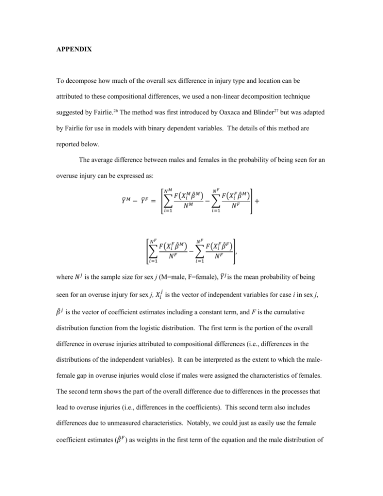
The average difference between males and females in the probability of being seen for an
overuse injury can be expressed as:
𝑁𝑀
𝐹
𝑖=1
𝑖=1
𝑁
𝐹(𝑋𝑖𝑀 𝛽̂ 𝑀 )
𝐹(𝑋𝑖𝐹 𝛽̂ 𝑀 )
𝑀
𝐹
̅
̅
𝑌 − 𝑌 = [∑
−
∑
]+
𝑁𝑀
𝑁𝐹
𝑁𝐹
𝐹
𝑖=1
𝑖=1
𝑁
𝐹(𝑋𝑖𝐹 𝛽̂ 𝑀 )
𝐹(𝑋𝑖𝐹 𝛽̂ 𝐹 )
−
∑
[∑
],
𝑁𝐹
𝑁𝐹
where 𝑁𝑗 is the sample size for sex j (M=male, F=female), 𝑌̅𝑗 is the mean probability of being
𝑗
seen for an overuse injury for sex j, 𝑋𝑖 is the vector of independent variables for case i in sex j,
𝛽̂ 𝑗 is the vector of coefficient estimates including a constant term, and F is the cumulative
distribution function from the logistic distribution. The first term is the portion of the overall
difference in overuse injuries attributed to compositional differences (i.e., differences in the
distributions of the independent variables). It can be interpreted as the extent to which the malefemale gap in overuse injuries would close if males were assigned the characteristics of females.
The second term shows the part of the overall difference due to differences in the processes that
lead to overuse injuries (i.e., differences in the coefficients). This second term also includes
differences due to unmeasured characteristics. Notably, we could just as easily use the female
coefficient estimates (𝛽̂ 𝐹 ) as weights in the first term of the equation and the male distribution of
independent variables (𝑋 𝑀 ) as weights in the second term. A third possibility is to weight the
first term of the decomposition with coefficient estimates from a pooled sample of males and
females. For the models in this paper, the choice of weights did not substantively alter our
conclusions, so for brevity’s sake we only report the results from the decompositions using the
pooled weights.
This technique estimates the total contribution of sex differences in the independent
variables to the male-female gap in the dependent variable. It also allows us to estimate the
separate contribution of each independent variable to the overall gap. Each contribution is equal
to the change in the mean predicted probability of the outcome from substituting the female
distribution with the male distribution of a specific variable, holding the distributions of the other
variables constant.
To compute the separate contributions, we follow Fairlie’s recommendation,26 pooling
the male and female samples and computing the predicted probability of being seen for an
overuse injury for each male and female in the sample. Since 𝑁 𝑀 ≠ 𝑁 𝐹 , we draw a random
subsample of females equal to the size of the male group and match and rank the two groups
based on their predicted probabilities. The results are sensitive to the subsample chosen; we thus
draw 1,000 different subsamples and base our results on average values obtained from
decompositions carried out over these subsamples. The decomposition estimates are also
sensitive to the ordering of the variables in the equation. We therefore randomize the order of the
variables across the simulations. We use the ‘fairlie’ command in Stata to compute both
estimates and standard errors, the latter of which are approximated using the delta method.26