NA1C0012
Jenny
11.5.2
ScentenceAccent with sex
ScentenceAccent with status
5
6
6
38
5
1
1
2
2
3
4
sentenceaccent
4
3
sentenceaccent
36
Female
Male
Non
sex
Late
Early
status
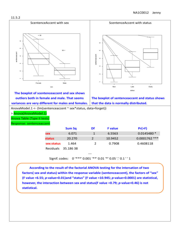
The boxplot of scentenceaccent and sex shows
outliers both in female and male. That seems
variances are very different for males and females.
The boxplot of sentenceaccent and status shows
that the data is normally distributed.
AnovaModel.1 <- (lm(sentenceaccent ~ sex*status, data=forget))
> Anova(AnovaModel.1)
Anova Table (Type II tests)
Response: sentenceaccent
Sum Sq
sex
6.071
status
20.270
sex:status
1.464
Residuals 35.186 38
Df
1
2
2
F value
6.5563
10.9452
0.7908
Pr(>F)
0.0145480 *
0.0001762 ***
0.4608118
--Signif. codes: 0 '***' 0.001 '**' 0.01 '*' 0.05 '.' 0.1 ' ' 1
According to the result of the factorial ANOVA testing for the intersation of two
factors( sex and status) within the response variable (sentenceaccent), the factors of “sex”
(F value =6.55; p-value=0.01)and “status” (F value =10.945; p-value=0.0001) are statistical,
however, the interaction between sex and status(F value =0.79; p-value=0.46) is not
statistical.
> numSummary(forget[,"sentenceaccent"], groups=forget$sex, statistics=c("mean", "sd", "IQR",
"quantiles"), quantiles=c(0,.25,.5,.75,1))
mean
sd
IQR
0% 25%
50%
75% 100%
data:n
Female 3.750000 1.207884 1.5000
Male 2.238636 1.011581 0.9375
1.375 2.875 3.625
1.000 1.500 2.125
4.3750
2.4375
6.75
4.75
33
11
> numSummary(forget[,"sentenceaccent"], groups=forget$status, statistics=c("mean", "sd", "IQR",
"quantiles"), quantiles=c(0,.25,.5,.75,1))
mean
sd
IQR
0%
25% 50%
75%
100%
data:n
Non
2.508333
1.0116141 1.7500
Late
3.100000
0.9344594
Early
4.589286
1.1152662
1.000 1.50000
2.625
3.25000
4.375
1.625 2.31250
2.875 3.75000
4.875
15
.2500 2.875 3.90625
4.750 5.15625
6.750
14
1.4375
15
From the mean scores of gender, we can see the females performed statistically better than
males. But for the result of status, we only can see the Early group is the best of three groups , the
Late group is in the middle and the Non group is the worst.
※posthoc
summary(.Pairs) # pairwise tests
Simultaneous Tests for General Linear Hypotheses
Multiple Comparisons of Means: Tukey Contrasts
Fit: aov(formula = sentenceaccent ~ status, data = forget)
Linear Hypotheses:
Estimate Std.
Error
t value
Late - Non == 0
0.5917
0.3727 1.587
Early - Non == 0
2.0810
0.3793 5.486
Early - Late == 0
1.4893
0.3793 3.926
--Signif. codes: 0 '***' 0.001 '**' 0.01 '*' 0.05 '.' 0.1 ' ' 1
Pr(>|t|)
0.263
<0.001 ***
<0.001 ***
(Adjusted p values reported -- single-step method)
The posthoc test shows that the group of “Late-Non” is not statistic, but the other two
groups”Early-Non” and “Early-Late” are statistic. Hence, we can say that Early group did the best
of all.
※ggplot
attach(forget)
forget
ggplot(forget,aes(x=status,y=sentenceaccent,fill=sex))+
geom_bar(stat="identity",width=0.5,color="black",position="dodge")
From the ggplot of the data”forget”, we can see no matter in “Non”,”Late”or “Early”, females
have the better performance than males. Furthermore, foucsed on the result of status visually, here the
overall performance of “Early Group” is better than the orther two groups.
11.5.3
Anova Table (Type II tests)
Response: score
Sum Sq
272.25
1599.74
236.30
806.30 90
Df
1
4
4
F value
30.389
44.641
6.594
Pr(>F)
3.342e-07 ***
< 2.2e-16 ***
0.0001062 ***
agegroup
task
agegroup:task
Residuals
--Signif. codes: 0 '***' 0.001 '**' 0.01 '*' 0.05 '.' 0.1 ' ' 1
Pairwise comparisons using t tests with pooled SD
data: score and task
Rhyming
Adjective
Imagery
Intention
Counting
0.6718
2.0e-06
1.5e-10
3.2e-11
Counting vs. Intention  most significant
Rhyming
Adjective
9.7e-06
8.5e-10
0.0369
1.2e-10
0.0098
Imagery
0.6466
Counting vs. Rhymingnot significant
Imagery vs. Intentionnot significant
Old:Rhyming
Old:Adjective
Old:Imagery
Old:Counting Old:Rhyming Old:Adjective Old:Imagery Old:Intention
0.94061
0.00542
0.00449
1.6e-05
1.3e-05
0.09542
-
Old:Intention
Young:Counting
Young:Rhyming
Young:Adjective
Young:Imagery
Young:Intention
0.00059
0.74264
0.70185
3.0e-07
3.9e-11
5.8e-15
Old:Rhyming
Old:Adjective
Young:Counting Young:Rhyming Young:Adjective Young:Imagery
Adjective vs. Intention or Imagery is originally significant
-
Old:Imagery
Old:Intention
Young:Counting
Young:Rhyming
Young:Adjective
Young:Imagery
Young:Intention
0.47698
6.8e-08
9.1e-12
2.9e-15
0.00048
0.78317
0.66106
2.3e-07
3.2e-11
5.8e-15
0.51409
0.00197
0.01800
0.00812
9.9e-06
2.8e-09
Applying post hoc
0.35338
4.2e-06
8.6e-05
0.35338
0.00370
4.2e-06
the intention they will have)
Adjective vs. Imagerynot significant
1.9e-06
2.8e-10
0.05198
3.7e-14
0.00017
0.00017
0.00241
0.05198
0.00014
6.8e-08
-
Adjective vs. Old:Intentionnot significant (the more the age, the less
0.06000