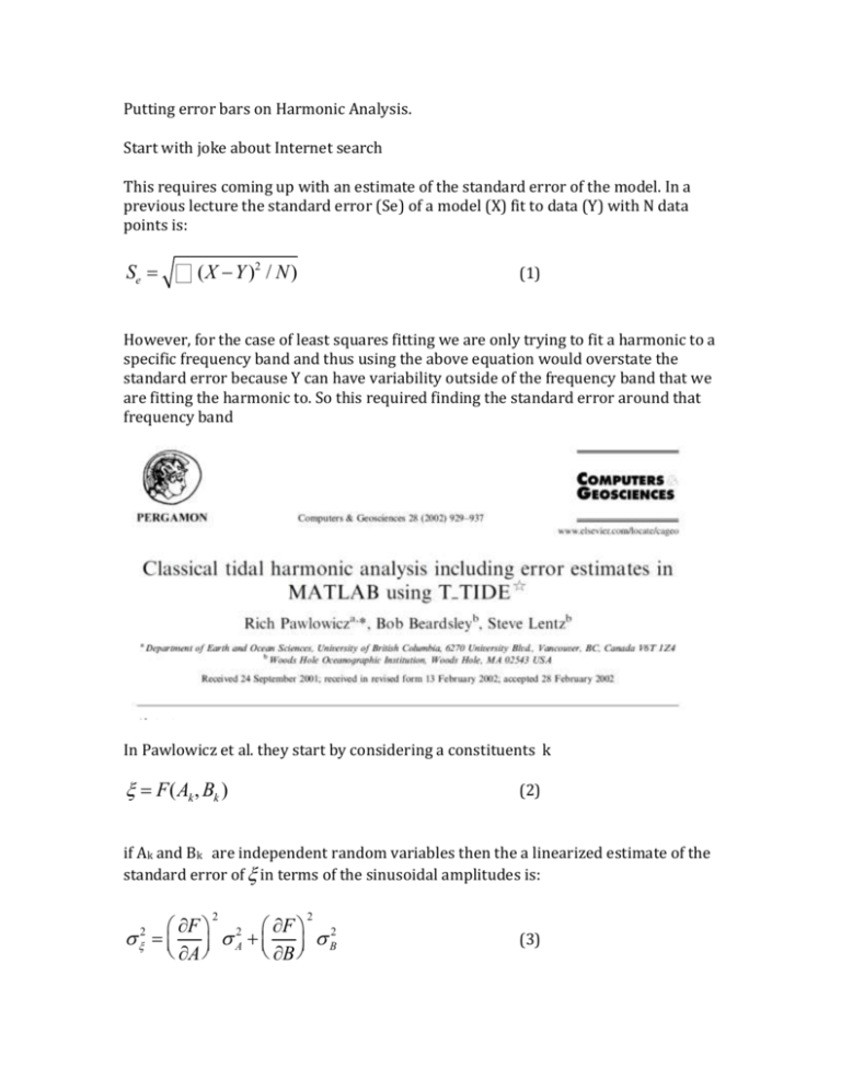
Putting error bars on Harmonic Analysis.
Start with joke about Internet search
This requires coming up with an estimate of the standard error of the model. In a
previous lecture the standard error (Se) of a model (X) fit to data (Y) with N data
points is:
Se =
å (X - Y )
2
/ N)
(1)
However, for the case of least squares fitting we are only trying to fit a harmonic to a
specific frequency band and thus using the above equation would overstate the
standard error because Y can have variability outside of the frequency band that we
are fitting the harmonic to. So this required finding the standard error around that
frequency band
In Pawlowicz et al. they start by considering a constituents k
x = F(Ak , Bk )
(2)
if Ak and Bk are independent random variables then the a linearized estimate of the
standard error of x in terms of the sinusoidal amplitudes is:
æ ¶F ö
æ ¶F ö
s x = ç ÷ s A2 + ç ÷ s B2
è ¶A ø
è ¶B ø
2
2
2
(3)
Here the standard error of the A’s and B’s (i.e. the ’s on the left hand side) are
obtained by the energy in the spectrum in the vicinity of the fitting frequency after
the harmonic has been removed. They also assume that A and B are equal.
Unfortunately in the paper they suggest that the partial differentials can be exactly
but tediously derived from equations 7-10 in the paper—which at first glance
contain now A’s or B’s.
I think an easier way to do this would be:
¶F / ¶A = (A 2 + B 2 )-1/2 A
2 -1/2
¶F / ¶B = (A + B )
2
(4ab)
B
Another way to proceed is what’s akin to a “Boot strap method”. Here we run a
Monti-Carlo simulation of a harmonic with the correct amplitude + ambient noise
and get the standard error of the amplitude and phase from those fits.
So here’s the procedure.
1) First get your harmonic fit.
2) remove harmonic(s) from time series
3) calculate fft of (2)
4) generate synthetic time series with harmonic from (1) and noise consistent with
the noise in the around the frequency band that you fit to in (3).
How do we do this?
Recall Parseval’s Theorem, which for using MATLAB X=fft(x) can be written us
å xx =
1
XX *
å
n
(5)
So if x is normally distributed noise with zero mean and a standard deviation then
the mean value is simply the chi-squared mean for one degree of freedom which is
one.
So if we call xg a normally distributed random variable with zero mean and a
standard deviation of one and we let our variable x=Dxg then the left hand side of 5
is simply nD2 . Defining Y=XX* (5) can be rewritten as:
D2 =
1
Y
Y
=
å
n2
n
Where Y is the mean across spectral bands. Thus to get the necessary amount of
noise for the Monti-Carlo simulation set
D = Y ±w / n
Where
to:
Y ±w is the mean value of Y around the frequency  that the harmonic was fit
So to proceed with error bars generated a synthetic time series
n=length(t);
x=A*sin(t)+Bcos(t)+D*normrnd(0,1,length(tm),1);
then perform harmonic analysis on x and calculate amplitude and phase.
Do this several hundred time (code T_TIDE does it 300) and from this you can
estimate the standard deviation of the amplitude, the standard deviation of the
phase and the 95% confidence limits are then simply 1.96 times this value.
In Class Exercise:
File data.mat has two time series that contain both noise (in this case auto
correlated red noise) plus several harmonics.
1) Load and plot mystery.m. tm it time in days. Are there any clear harmonics?
2) Use fft to find frequencies of any clear peaks. How many? What periods?
3) Use lsq to estimate the amplitude and phase of each Harmonic
4) Use dmod to plot the time varying amplitude of each group of harmonics
5) Remove harmonics from raw data
6) Plot spectra of data with harmonic removed.
7) Estimate error statistics for each set of harmonic
8) Run Monti-Carlo simulations to generate statistics of fits for each harmonic
9) Put 95% error bars on each estimate of amplitude and phase.