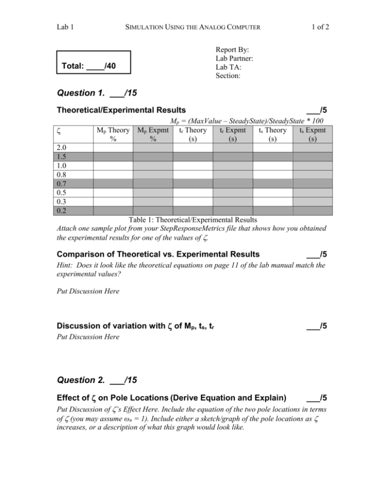
Lab 1
SIMULATION USING THE ANALOG COMPUTER
1 of 2
Report By:
Lab Partner:
Lab TA:
Section:
Total: ____/40
Question 1. ___/15
Theoretical/Experimental Results

Mp Theory
%
Mp Expmt
%
___/5
Mp = (MaxValue – SteadyState)/SteadyState * 100
tr Theory
tr Expmt
ts Theory
ts Expmt
(s)
(s)
(s)
(s)
2.0
1.5
1.0
0.8
0.7
0.5
0.3
0.2
Table 1: Theoretical/Experimental Results
Attach one sample plot from your StepResponseMetrics file that shows how you obtained
the experimental results for one of the values of .
Comparison of Theoretical vs. Experimental Results
___/5
Hint: Does it look like the theoretical equations on page 11 of the lab manual match the
experimental values?
Put Discussion Here
Discussion of variation with  of Mp, ts, tr
___/5
Put Discussion Here
Question 2. ___/15
Effect of  on Pole Locations (Derive Equation and Explain)
___/5
Put Discussion of ’s Effect Here. Include the equation of the two pole locations in terms
of  (you may assume ωn = 1). Include either a sketch/graph of the pole locations as 
increases, or a description of what this graph would look like.
Lab 1
SIMULATION USING THE ANALOG COMPUTER
2 of 2
Effect of Pole Locations on Mp, ts, tr for an Underdamped System
___/5
Hint: An underdamped system has  ____
As  increases, the poles do____ which makes Mp, ts, tr do _______
(Double Hint: moving the poles causes two different effects on ts)
Effect of Pole Locations on Mp, ts, tr for an Overdamped/Critically
Damped System
___/5
Hint: An over-damped system has  ____
A critically damped system has  ____
As  increases, the poles do____ which makes Mp, ts, tr do _______
Question 3. ___/10
Investigate the effects of approximating an overdamped 2nd order system with a 1st order
system. The approximation will be done by using a transfer function with only the pole
that is closer to the origin, pmin.
p1 p2
pmin
H1 ( s ) 
 H 2 (s) 
( s  p1 )( s  p2 )
s  pmin
Similarities/Differences on Overdamped 2nd-Order system to a 1stOrder System with the less negative of the 2nd-Order’s poles
___/6
Plot the step responses for the 2nd order systems and their 1st order approximations for
 = 1.5,  = 5, and  = 40. Assume ωn = 1. How are the step responses of the 1st order
approximations similar to and different from the step responses of the original 2nd order
systems?
Effect of magnitude of  on the accuracy of the approximations ___/4
How does  affect the accuracy of the 1st order approximations?
Attachments (3)



Plots obtained during lab
Sample response with relevant points for calculating Mp, ts and tr marked
Step Responses comparing 2nd order systems and 1st order approximations