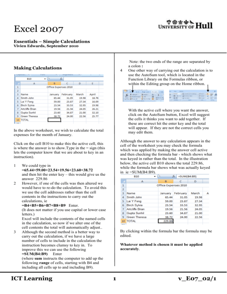
Excel 2007
Essentials – Simple Calculations
Vivien Edwards, September 2010
Making Calculations
4
With the active cell where you want the answer,
click on the AutoSum button, Excel will suggest
the cells it thinks you want to add together. If
these are correct hit the enter key and the total
will appear. If they are not the correct cells you
may edit them.
In the above worksheet, we wish to calculate the total
expenses for the month of January.
Although the answer to any calculation appears in the
cell of the worksheet you may check the formula
which was applied by making the answer cell active
and then checking the formula bar - which shows what
was keyed in rather than the total. In the illustration
below, the active cell B10 shows the total 229.86,
while the formula bar shows what was actually keyed
in ie =SUM(B4:B9).
Click on the cell B10 to make this the active cell, this
is where the answer is to show.Type in the = sign (this
lets the computer know that we are about to key in an
instruction).
1
2
3
We could type in
=65.44+59.00+23.54+19.56+23.60+38.72
and then hit the enter key – this would give us the
answer 229.86
However, if one of the cells was then altered we
would have to re-do the calculation. To avoid this
we use the cell addresses rather than the cell
contents in the instructions to carry out the
calculations, ie
=B4+B5+B6+B7+B8+B9 Enter.
(It does not matter if you use capital or lower case
letters.)
Excel will include the contents of the named cells
in the calculation, so now if we alter one of the
cell contents the total will automatically adjust..
Although the second method is a better way to
carry out the calculation, if we have a large
number of cells to include in the calculation the
instruction becomes clumsy to key in. To
improve this we can use the following
=SUM(B4:B9) Enter
(where sum instructs the computer to add up the
following range of cells, starting with B4 and
including all cells up to and including B9).
ICT Learning
Note: the two ends of the range are separated by
a colon :
One other way of carrying out the calculation is to
use the AutoSum tool, which is located in the
Function Library on the Formulas ribbon, or
within the Editing group on the Home ribbon.
By clicking within the formula bar the formula may be
edited.
Whatever method is chosen it must be applied
accurately.
1
v_E07_02/1
2. Select (highlight) the cells you wish to apply the
copied formula to(C10 to E10) and then click on
the paste button in the Clipboard area of the Home
ribbon. Or, select the cells (C10 to E10) and then
right click over them and choose Paste from the
pop-up menu.
Calculations Other Than Addition
If we need to make different sorts of calculations we
need to use different symbols
subtract
-
(=A4-A5)
multiply
*
(=A4*A5)
divide
/
(=A4/A5)
Alternatively, the fill box may be used
With cell B10 active, take the mouse pointer to the
bottom right-hand corner of the cell, where a small
black box is visible. If the pointer is in the correct
position it will change to a thin black cross (hairline).
Hold down the left mouse key and drag across the cells
which you wish to receive the formula (C10 to E10).
When you release the mouse button the cells will
contain the total values for the other months.
BODMAS
This is the order in which calculations will be carried
out if a formula contains more than one mathematical
symbol. It stands for
Brackets, Order, Division, Multiplication,
Addition, Subtraction
So, in the formula
=1+2*3
the answer is 7
(2 is multiplied by 3 and then the 1 is added)
If we had wanted it calculated so that 1 and 2 are
added before being multiplied by 3, we would need to
have used brackets around the first step of the
calculation, thus
To Show Formulae in the Worksheet
= (1 + 2) * 3
giving the answer
9
(1 is added to 2 and the result is then multiplied by 3)
If you wish to check a formula in an individual cell,
clicking on the cell will show the formula in the
formula bar. However, it is possible show all formulae
used in a spreadsheet rather than the values they
produce. To do this
Replicating Formulae
Once a formula has been applied in a cell it can be
copied to other cells requiring the same calculation.
Hold down the Control key (Ctrl) on the keyboard and
hit the grave accent key (the leftmost key on the
number row at the top of the keyboard, below Esc).
This will toggle between showing formulae and values.
In the previous example, we have calculated the total
expenses for January. Rather than keying in the
formulas to total expenses for February, March and
April we can apply the formula we created for January
to the total cells for those months.
1.
Note that when in formulae view columns may need to
be widened to show the full formulae. If you are
printing it may be advisable to turn the paper to
landscape.
Make cell B10 the active cell, then, in the Clipboard
group to the left of the Home ribbon, click on the
Copy button. Alternatively, you may right click
over the selected cell and choose Copy from the
pop-up menu
ICT Learning
2
v_E07_02/1