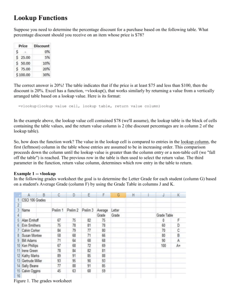
Lookup Functions
Suppose you need to determine the percentage discount for a purchase based on the following table. What
percentage discount should you receive on an item whose price is $78?
The correct answer is 20%! The table indicates that if the price is at least $75 and less than $100, then the
discount is 20%. Excel has a function, =vlookup(), that works similarly by returning a value from a vertically
arranged table based on a lookup value. Here is its format:
=vlookup(lookup value cell, lookup table, return value column)
In the example above, the lookup value cell contained $78 (we'll assume), the lookup table is the block of cells
containing the table values, and the return value column is 2 (the discount percentages are in column 2 of the
lookup table).
So, how does the function work? The value in the lookup cell is compared to entries in the lookup column, the
first (leftmost) column in the table whose entries are assumed to be in increasing order. This comparison
proceeds down the column until the lookup value is greater than the column entry or a non-table cell (we "fall
off the table") is reached. The previous row in the table is then used to select the return value. The third
parameter in the function, return value column, determines which row entry in the table to return.
Example 1 -- vlookup
In the following grades worksheet the goal is to determine the Letter Grade for each student (column G) based
on a student's Average Grade (column F) by using the Grade Table in columns J and K.
Figure 1. The grades worksheet
To determine the Letter Grade for the first student, Alan Emhoff in row 5, we must determine the three
parameter values to use in the vlookup function:
=vlookup(lookup value cell,
lookup table,
return value column)
The parameters are:
1. lookup value cell -- cell that contains the value in the worksheet we want to lookup -- the Average Grade
in column F, so cell F5.
2. lookup table -- the table of lookup values -- the Grade Table values in the block J5:K10
3. return value column -- the column number in the lookup table that contains the value to be returned -the letter grade in the Grade Table is in column 2.
Since we want to copy the formula to determine the Letter Grade for all students, we need to use an absolute
reference for the Grade Table (the table has a fixed location) and our formula for Alan Emhoff becomes:
=vlookup(F5,$J$5:$K$10,2)
Example 2 -- vlookup with the lookup table on separate worksheet
This example provides two interesting features: the lookup occurs within a calculation and the lookup table is
on a separate worksheet in the same workbook. First, let's discuss the problem. The primary worksheet for the
problem is shown below.
Figure 2. The main Union employees worksheet
The first computation finds of the union pay rate which is placed in column E. The union pay rate depends upon
two factors: the years of experience and the shift the employee works. The first factor, years of experience, is
the value used as the lookup value in the lookup table. Note in Figure 3 below the leftmost column in the lookup
table on the RateTab worksheet is years of experience. This lookup provides the base rate for the salary.
Figure 3. RateTab worksheet containing the lookup table for the union pay computation worksheet
To get the shift increment an =if() needs to be used (since the increment depends on the shift). There are three
shifts which means three cases, so one of the actions of the =if() function is a second =if() function. For
example, with the first condition we check whether the shift is 1 or not. If the answer is yes, then the increment
is 0. If the answer is no, then two shifts (2 and 3) remain and a test to check if it's 2 or 3 is required. The
formula in cell E7 to determine the shift increment would then have the form:
=if(D7=1, 0, if(D7=2, $L$4, $L$5)).
Note: When there are three alternatives there needs to be two =if() functions. The first determines if the shift is
1. If it is not, then the shift must be 2 or 3 which are the true and false cases of the second if.
To refer to an object, in this case our lookup table, on another worksheet the name of the worksheet needs to be
indicated before making the reference. When there are no embedded blanks in the worksheet name as in this
worksheet one types RateTab!.
If the worksheet has a name such as Sept Sales, which contains a blank between the 't' in Sept and the 'S' in
Sales the reference has the form 'Sept Sales'!.
Of course, one can always use the apostrophes even if there are no blanks; there is no harm in typing
'RateTab'!.
Now, to make the calculation for the union pay rate (base rate + shift differential) enter:
=vlookup(C7,RateTab!$B$6:$C$12,2) + if(D7=1, 0, if(D7=2, $L$4, $L$5))
To complete the worksheet, the gross pay is computed as the product of the union pay rate and the number of
hours worked.
Example 3 -- vlookup with a data element determining the column to retrieve
This simple worksheet contains yearly payroll data. The columns contain employees, taxable income, and the
number of deductions for the employee. The primary worksheet is shown below. There are two columns for
which calculations need to be made, the taxes due and the net income.
Figure 4 The main worksheet for tax computation example.
The lookup table is contained on the worksheet taxtable1 shown below in Figure 5.
Figure 5. The taxtable1 worksheet for this example.
Column A is the lookup column containing salary cutoffs and columns B through F contain taxes due for the
number of deductions ranging from 0 to 4. The tax amount to retrieve depends upon on the employee's salary
bracket and the number of deductions. This dependency is what makes determining the third parameter
interesting. If an employee has 0 deductions, then the tax is contained in column B, the second column in the
table. Note that the 2 (column number for the second column) is the number of deductions, 0 for Alan Emhoff,
plus 2. Similarly, if an employee has 3 deductions, then the tax is contained in column E, column 5 of the table.
Again, the column number of the return value is 2 more than the number of deductions. So, the third parameter
in the =vlookup() for the first employee, Alan Emhoff, is C5 + 2. The complete =vlookup function to use in cell
D5 is:
=vlookup(B5,taxtable1!$A$3:$F$7,C5+2)
The function will then be copied to the range D6:D8. The Net Income will be the Taxable Income less the
Taxes Due. This formula is copied down column E.
Example 4 -- another tax table vlookup
In this example the primary worksheet from the previous section is again used. The table on the worksheet
taxtable1 in Figure 6 below is a graduated tax table -- its leftmost column is B, the lookup column, which
contains taxable income. In column B are the lower bounds of the tax brackets. The brackets are [0, 9999.99],
[10000, 29999.99], …, [100000, all other larger incomes].
Figure 6 The taxtable1 worksheet for a second type of tax calculation.
To compute the tax using the graduated tax rate table, you first need the value of the base tax for the bracket.
Let's suppose the taxable income is 63000. Then the required tax bracket is [30000, 69999.99]. For this bracket
there is a base tax of 3000. To compute the tax for the income exceeding 30000, first calculate the excess over
the lower bracket limit: 63000 - 30000; in this case the excess equals 33000. The tax rate for this bracket is
12%. So, the tax on the excess is 33000 * 0.12 = 3960. The tax due for the taxable income of 63000 is the base
tax plus the tax on the excess or 3000 + 3960 = 6960. Note that this calculation requires three vlookups: one to
find the base tax, a second to find the lower bracket limit to compute the excess taxable income, and a third to
find the tax rate for the tax bracket of the total taxable income. The vlookup for the base tax is:
=vlookup(B5,taxtable1!$B$5:$D$9,2).
The calculation of the excess taxable income is:
=B5 - vlookup(B5,taxtable1!$B$5:$D$9,1).
The calculation of the tax on the excess income is:
=vlookup(B5,taxtable1!$B$5:$D$9,3) *( B5 - vlookup(B5,taxtable1!$B$5:$D$9,1)).
Notice the need for the parenthesis around the calculation of the excess taxable income. Recall that the rate
applies to the excess taxable income.
Example 5 -- vlookup when the lookup column is unordered (need to specify a 4th parameter for
vlookup)
When the lookup column is unordered the lookup value needs to be an exact match with a value in the lookup
column. In this case, a fourth parameter is needed for the =vlookup() function that has the value FALSE. In
general, the fourth parameter is the default value TRUE and does not need to be entered when the lookup
column is in increasing order.
The following table in Figure 7 shows currency conversion ratios for the currency units of several countries
versus the US dollar.
Figure 7. Currency conversion ratios
The table is used to convert a given number of dollars to a number of units in a given country's currency. That
is, the user enters the country to which they are travelling and the amount of US currency that is being
exchanged and the vlookup function returns the number of currency units that can be obtained. Note that the
leftmost column, the lookup column, in the table is the country and the countries are not in alphabetical order in
the country listing.
The vlookup functions with their necessary arguments are shown below in the primary worksheet calculator in
Figure 8. Note the use of FALSE as the fourth parameter to indicate the country must be matched exactly.
Figure 8. The model for the main worksheet for the currency conversion problem.
Example 6 -- The horizontal lookup function =hlookup
The =hlookup function can be used when tables are horizontally arranged, such as the following lookup table in
Figure 9.
Figure 9. Horizontal lookup table
Based on the Excel spreadsheet above:
=hlookup(10112,
=hlookup(10112,
=hlookup(10109,
=hlookup(10109,
More Exercises
Vlookup
C2:G4,
C2:G4,
C2:G4,
C2:G4,
2,
3,
2,
2,
FALSE) would return $6.00
FALSE) would return 12
FALSE) would return #N/A
TRUE) would return $11.00