Electronic Supplementary Material for:
“Potential consequences of climate change for primary production and fish production in large marine ecosystems”
Julia L. Blanchard 1,2* , Simon Jennings 3,4 , Robert Holmes 5 , James Harle 6 , Gorka Merino 5 , Icarus
Allen 5 , Jason Holt 6 , Nicholas K. Dulvy 7 & Manuel Barange 5
A. Model Equations and Parameters
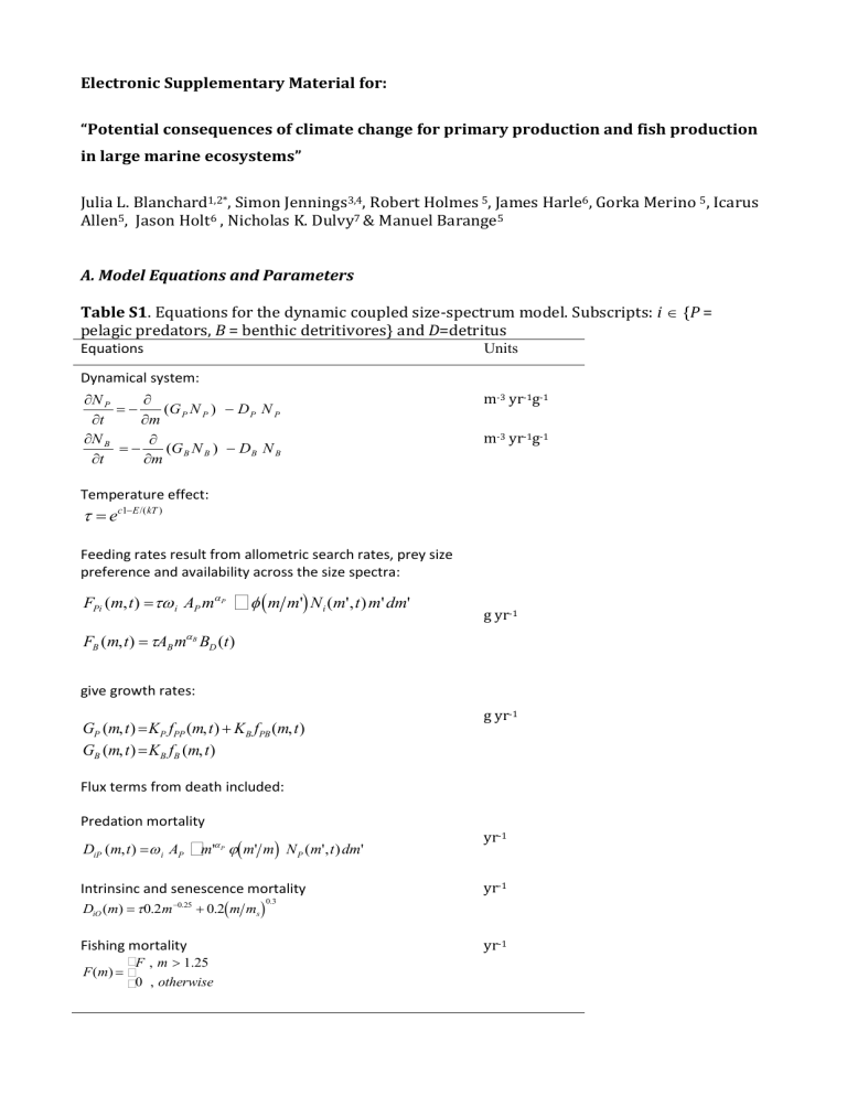
Table S1. Equations for the dynamic coupled size-spectrum model. Subscripts: i  {P = pelagic predators, B = benthic detritivores} and D=detritus
Equations Units
Dynamical system:

N
 t
P

N
 t
B





 m

 m
( G
( G
P
N
P
B
N
B
)
)
Temperature effect: t = e c 1
-
E /( kT )

D
P

D
B
N
P
N
B
Feeding rates result from allometric search rates, prey size preference and availability across the size spectra:
F
Pi
( m , t )
= tw i
A
P m a
P
f ( m m
)
' N i
( m ', t ) m ' d m '
F
B
( m , t )
= t
A
B m a
B B
D
( t ) m -3 yr -1 g -1 m -3 yr -1 g -1 g yr -1 give growth rates:
G
P
G
B
( m , t )
=
K
P
( m , t )
=
K
B f f
PP
( m , t )
+
K
B
B
( m , t ) f
PB
( m , t )
Flux terms from death included: g yr -1 yr -1
Predation mortality
D iP
( m , t )
= w i
A
P
m ' a
P j ( m ' m
)
N
P
( m ', t ) dm '
Intrinsinc and senescence mortality
D iO
( m )
= t
0.2
m
-
0.25
+
0.2
( m m s
)
0.3
Fishing mortality
F ( m )
=   í
F
,  m
>  1.25
0  ,  otherwise yr -1 yr -1

Total death rates were:
D i
( m , t )
=
D iP
( m , t )
+
D iO
( m )
+
F ( m )
Fishing mortality was only applied to the pelagic community where F was equal across all size > 1.25 g and the value of F was varied. yr -1

Table S2. Parameter definitions, values and units for the dynamic coupled size spectrum model. In cases where two values are given the first value is for pelagic predators and the second value is for benthic detritivores.
Symbol Definition Value Unit m min m
P,min minimum body mass of plankton minimum body mass of pelagic predators
10
10
-12
-3 g g m
B,min
(also of max body size of plankton) minimum body mass of benthic 10 -3.5
detritivores maximum body size in the whole system. 10 6 g m max g k
E c1

β
σ
Boltzmann constant activation energy constant preference for prey in either the pelagic or benthic spectrum preferred predator-prey mass ratio log10(PPMR) measure of the width of the log10 PPMR distribution pre-factor of search volume A

K exponent of search volume net growth conversion efficiency z z i
0 pre-factor for background mortality exponent for intrinsic background mortality start size for senescence mortality m s z s exponent for senescence background mortality
B. Model application and output
8.62E-5 eV K -1
0.63 eV
25.55
0.5
2.0
1.0
64, 6.4

0.2, 0.1
0.1
-0.25
1
0.3 m 3 kg
yr yr -1 g yr -1 g yr -1
-1
The plankton size spectrum is not modelled explicitly but has temporal dynamics that are driven by output from a coupled physical-biogeochemical model, POLCOMS-ERSEM. Temporal changes in the intercept of the plankton component of size-spectrum were estimated from phytoplankton and microzooplankton biomass density. The plankton size spectrum was described as log N(m) = a + blog(m) where N is abundance density per unit volume at mass, and mass is m (in grams). We estimate a from the total biomass density of phytoplankton and microzooplankton functional groups from the physical-biogeochemical model output by spreading the density across a realistic size range (10 -14 to 10 -4 g) and assuming a fixed slope
b of -1, in keeping with global empirical studies of phytoplankton size spectra [38]. Near sea floor detritus biomass density estimates from the physical-biogeochemical model were used

to force the detritus dynamics. Temperature estimates were taken form the mixed layer depth and near sea floor vertical layers for the pelagic predators and benthic detritivores, respectively.
The total biomass density (g m -3 ) across a size-range (m1=1 g to m2= 100 kg) was computed from the predicted numerical density at size N(m) at time across the continuum of body masses m as: m 2 m 1
ò
N ( m ) mdm
(1)
Similarly, the total fish production (g m -3 yr -1 ) was calculated from the growth rates at size
G(m) and the numerical density at size: m 2 ò m 1
G ( m ) N ( m ) dm
(2)
The total annual catch (or ‘yield’, in g m -3 yr -1 ) across a size-range was calculated by combining
(1) with the fishing mortality rate at size
F ( m )
: m 2 ò m 1
F ( m ) N ( m ) mdm
(3)

C. Details of the large regional marine ecosystem domains
Table S3. The large regional domains of coastal and shelf seas included in the analysis and the corresponding Large Marine Ecosystems (LME) that make up the domains, with information on the primary production, surface area and 2005 fish catches. These 28 LMEs contributed approximately 77% of the landed catch from all LMEs combined around the world, and 60% of the global marine landed catches.
PP Area Fish Catch 2005
Domain LME
Bengal Bay of Bengal
Benguela Benguela Current
(mgC.m
-2 .d
-1 )
729
1,387
(10 3 .km
2)
3,657
1,470
(t)
3,818,679
1,095,408
Canary
Guinea
Canary Current
Guinea Current
Humboldt Humboldt Current
Indo-
Yellow Sea
Pacific
Indo-
Pacific
Indo-
Pacific
South China Sea
Sulu-Celebes Sea
1,196
980
876
1,613
477
573
1,120
1,959
2,619
439
5,662,985
1,016
2,077,314
859,111
9,855,464
2,063,739
6,606,620
1,111,075
Indo-
Pacific
Indo-
Pacific
Indonesian Sea
Gulf of Thailand
NW Pacific East China Sea
NW Pacific Kuroshio Current
NW Pacific Okhotsk Sea
NW Pacific Oyashio Region
Sea of Japan/ East
NW Pacific Sea
NE Atlantic North Sea
NE Atlantic Celtic Biscay Shelf
NE Atlantic Faroe Plateau
NE Atlantic Iberian Coastal
NW
Atlantic
NW
Atlantic
NW
Newfoundland-
Labrador
NE US Continental
Shelf
Atlantic
Nordic
Nordic
Nordic
Nordic
Scotian Shelf
Norwegian Shelf
Icelandic Shelf
Greenland Sea
Baltic Sea
California California Current
California Gulf of California
772
780
891
422
815
716
604
1,115
956
422
758
809
1,536
1,395
491
551
477
1,910
613
1,199
2,289,597
391,665
1,008
1,333,074
1,627
664
1,054
690,041
766,550
151
301
675
308
413
1,109
521,237
1,176
397
2,225
216
1,609,263
862,066
3,329,876
612,605
2,662,794
584,048
1,166,937
1,885,726
1,086,603
316,817
299,644
354,768
741,834
351,017
1,341,406
1,312,248
127,504
702,404
728,988
195,308

D. Model cross-validation
●
150
100
●
50
0
●
●
●
●
●
●
●
●
●
●
●
●
● ●
●
●
●
●
●
●
●
●
●
●
●
●
●
●
●
●
●
●
●
●●
●
●
●
●
●
●
●
●
●
●
●
●
●
●
●
●
●
●
●
●
●
●
●
●
●
●
−50
●
●
●
●
●
Domain
● Bay of Bengal
●
●
Benguela
Canary
●
●
●
Guinea
Humbolt
Indo−Pacific
●
●
●
●
●
NW Pacific
NE Atlantic
NW Atlantic
Nordic Shelf Seas
California Current
0 50 100
Static Model − predicted % change in biomass density
Figure S1. Comparison of predicted percentage changes (climate relative to control) in overall fish biomass density from the static metabolic scaling model and the dynamic coupled size spectrum model. Each point represents an EEZs group by colour according the large ecosystem domains (codes in legend). Solid line is 1:1 relationship.

E. Effect of fishing on fish production and resilience to climate change across ecosystems.
B en ga l
B en gu el a
C an ar y
G ui ne a
H um bo lt
In do
−P ac ifi c
N
W
P ac
N
E
A tl
N
W
A tl
N or di c
S ea s
C al ifo rn ia a) climate, no fishing climate, low fishing climate, high fishing b)
Figure S2. Climate-projected changes in (a) large fish production and (b) Coefficients of
Variation (CVs) of large fish biomass density time series. Changes are relative to the unexploited control scenario when fishing mortality rates are = 0 (dark grey, climate only),
0.2 (light grey, low fishing) and 0.8 yr -1 (white, high fishing) for all economic zones grouped by their 11 regional ecosystems domains.