Garg, Khan, Lu, Roberts, Tang, Tillu
1
Investigation of Long Memory in Quarterly
Home Price Index Data
Vikas Garg, Yasin Khan, Shirley Lu, Timothy Roberts, Yifan Tang, Wesley Tillu

Abstract—
…………………………………………………………………………
…………………………………………………………………………
…………………………………………………………………………
…………………………………………………………………………
…………………………………………………………………………
…………………………………………………………………………
…………………………………………………………….…………
…………………………………………………………………………
…………………………………………………………………………
…………………………………………………………………………
……………………………………………….………………………
…………………………………………………………………………
…………………………………………………………………………
…………………………………………………………………………
………………………………….……………………………………
…………………………………………………………………………
………………….
I. INTRODUCTION
I
N
A. Stationarity
2.1
B. Unit Root Non-Stationarity
C. ARCH Effect
B. Initial Analysis
1) Exploratory Data Analysis
2) Data Transformations
Many parameter estimators are based on the assumption of
Gaussian distribution. In particular, the Whittle estimator for
the fractional differencing parameter is one such estimator.
The Whittle estimator is generally preferred over other
fractional differencing parameters as it is consistent, unbiased,
and asymptotically efficient.
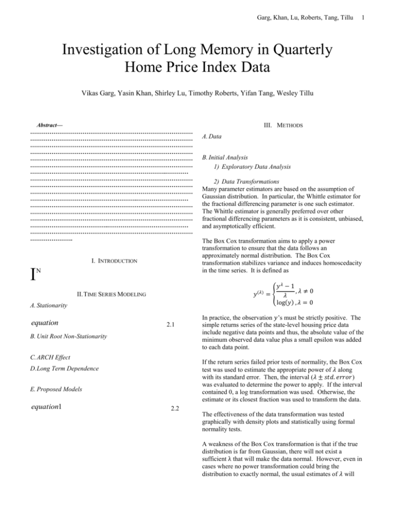
The Box Cox transformation aims to apply a power
transformation to ensure that the data follows an
approximately normal distribution. The Box Cox
transformation stabilizes variance and induces homoscedacity
in the time series. It is defined as
(𝜆)
𝑦𝜆 − 1
= { 𝜆 ,𝜆 ≠ 0
log(𝑦) , 𝜆 = 0
In practice, the observation 𝑦’s must be strictly positive. The
simple returns series of the state-level housing price data
include negative data points and thus, the absolute value of the
minimum observed data value plus a small epsilon was added
to each data point.
If the return series failed prior tests of normality, the Box Cox
test was used to estimate the appropriate power of 𝜆 along
with its standard error. Then, the interval (𝜆 ± 𝑠𝑡𝑑. 𝑒𝑟𝑟𝑜𝑟)
was evaluated to determine the power to apply. If the interval
contained 0, a log transformation was used. Otherwise, the
estimate or its closest fraction was used to transform the data.
D. Long Term Dependence
E. Proposed Models
equation1
A. Data
𝑦
II. TIME SERIES MODELING
equation
III. METHODS
2.2
The effectiveness of the data transformation was tested
graphically with density plots and statistically using formal
normality tests.
A weakness of the Box Cox transformation is that if the true
distribution is far from Gaussian, there will not exist a
sufficient λ that will make the data normal. However, even in
cases where no power transformation could bring the
distribution to exactly normal, the usual estimates of 𝜆 will
Garg, Khan, Lu, Roberts, Tang, Tillu
2
lead to a distribution that satisfies certain restrictions on the
first 4 moments, thus will be usually symmetric.
3) I(1) Testing
4) Normality Testing
C. Parameter Estimation for Model Building
1) Parametric vs Non Parametric vs Semi-parametric
2) Linear Time Series Parameters
3) Nonlinear Time Series Parameters
4) Fractional Differencing Parameters
5) Joint Estimation of ARFIMA Parameters
Figure 4.x: QQ plots and density plots of the Arkansas simple return
series (left) and the Box Cox transformed series with 𝝀=1.11 (right)
D. Model Checking and Performance
1) Absolute
2) Relative
IV. RESULTS
A. Initial Analysis
1) Exploratory Data Analysis
2) Data Transformations
Analysis of the states demonstrated that the distribution of the
returns deviates too far from Gaussian and thus, any Box Cox
transformation attempt fails. Figure 4.x shows graphical
results from before and after the transformation for Arkansas
and Table 4.x. shows numerical results.
p-value
Shapiro
JB
AD
KS
AR
1.75E-12
2.20E-16
2.20E-16
2.20E-16
AR Box Cox transformed
(λ = 1.11)
3.07E-12
2.20E-16
2.20E-16
2.20E-16
Table 4.x: p-values from normality tests for the Arkansas simple return
series and the Box Cox transformed series with 𝝀=1.11 (right)
The QQ plots and density plots show significant departures
from normality. The p-values of various normality tests
strongly suggest non-normal distributions. It is concluded that
a Box Cox transformation is inadequate in making the return
series Gaussian.
3) I(1) Testing
4) Normality Testing
B. Parameter Estimation for Model Building
1) Parametric vs Non Parametric vs Semi-parametric
2) Linear Time Series Parameters
3) Nonlinear Time Series Parameters
4) Fractional Differencing Parameters
5) Joint Estimation of ARFIMA Parameters
Garg, Khan, Lu, Roberts, Tang, Tillu
C. Model Checking and Performance
1) Absolute
2) Relative
D. Validity and Interpretation
V. CONCLUSION
ACKNOWLEDGMENT
REFERENCES
[1]
[2]
[3]
[4]
T. J. Barstow and Paul A. Mole. “Linear and nonlinear characteristics of
oxygen uptake kinetics during heavy exercise,” American Physiological
Society.
Stephen Steiler. “The Lactate Threshold.”
http://home.hia.no/~stephens/lacthres.htm
Stirling, J. R., Zakythinaki, M., Refoyo, I., and Sampedro, J. “A Model
of Hear Rate Kinetics in Response to Exercise.” Journal of Nonlinear
Mathematical Physics. Vol 15. 2008
Tsay, R. S. Analysis of Financial Time Series: Second Edition.
3