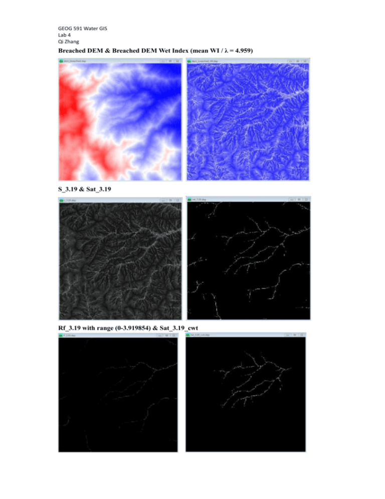
GEOG 591 Water GIS
Lab 4
Qi Zhang
Breached DEM & Breached DEM Wet Index (mean WI / λ = 4.959)
S_3.19 & Sat_3.19
Rf_3.19 with range (0-3.919854) & Sat_3.19_cwt
GEOG 591 Water GIS
Lab 4
Qi Zhang
Sat_3.19_cwt_area & cwt_mask_area
The total saturated area = 171900 m2, the catchment area = 1.61348 x 107 m2
So, Variable source area = 171900 / (1.61348 x 107) = 0.01065399
Part 1
Other 4 values of mean saturation deficit were selected, which together with 3.19 were:
2.51, 2.86, 3.19, 3.57, 3.82
The results showed below in the table 1.
Table 1 Values for different mean saturation deficit (m=0.4517)
Value #
1
2
mean saturation deficit
Total saturated area/m2
Catchment area/m2
Variable source area
2.51
2.86
333000
238600
1.61348 x 107
0.02063862 0.01478791
3
4
5
3.19
171900
3.57
126000
3.89
93900
0.01065399
0.00780921
0.00581672
VSA - Smean Plot (m=0.4517)
0.024
0.022
0.02
0.018
0.016
0.014
0.012
0.01
0.008
0.006
0.004
0.002
0
VSA
Linear (VSA)
y = -0.0105x + 0.0457
R² = 0.958
2.4 2.6 2.8
3
3.2 3.4 3.6 3.8
4
Fig. 1 Plot for VSA to Smean
4.2
GEOG 591 Water GIS
Lab 4
Qi Zhang
With the increase of mean saturation deficit, the VSAs decrease as an exponential trend.
This indicates that the total saturated area decreases as mean saturation deficit get higher,
which is associated with high sensitivity in lower level.
Part 2
Now 0.6289 has been selected for m value, and the same process was repeated. The results
showed below.
Table 1 Values for different mean saturation deficit (m=0.6289)
Value #
1
2
mean saturation deficit
Total saturated area/m2
Catchment area/m2
Variable source area
2.51
2.86
643300
505200
7
1.61348 x 10
0.03987
0.031311
3
4
5
3.19
403800
3.57
318600
3.89
253200
0.025027
0.019746
0.015693
VSA - Smean Plot (m=0.6289)
0.045
0.04
0.035
0.03
0.025
0.02
0.015
y = -0.0173x + 0.0816
R² = 0.9802
0.01
0.005
0
2.4
2.6
2.8
3
3.2
3.4
3.6
3.8
4
4.2
Fig. 2 Plot for VSA to Smean (m=0.6289)
Comparing with the previous plot, it was showed that VSA is obviously sensitive to m. If
higher value of m was set, VSAs also positively increase to higher values. This indicates that
higher value of m will lead to higher saturation area within a given catchment.
To provide visual comparison, two plots were combined into one graph and the difference
between these two trendlines thus better verify the results.
GEOG 591 Water GIS
Lab 4
Qi Zhang
VSA - Smean Plot for both m
0.048
0.044
0.04
0.036
0.032
0.028
0.024
0.02
0.016
0.012
0.008
0.004
0
VSA1
VSA2
y = -0.0173x + 0.0816
R² = 0.9802
y = -0.0105x + 0.0457
R² = 0.9580
2.4
2.6
2.8
3
3.2
3.4
3.6
3.8
4
4.2
Fig. 3 Plot for VSA to Smean for both m
Part 3 Maps for Si, return flows and saturated areas
The maps for Si, Saturated area, and Return flow are listed below,
Smean are 2.51, 2.86, 3.19, 3.57, 3.82, m =0.4517
Fig. a) Maps of Si (scale is from -4.599854 to 3.843346)
GEOG 591 Water GIS
Lab 4
Qi Zhang
Fig. b) Maps of saturated areas (scale is 0/1)
Fig. c) Maps of return flow (scale is from -1 to 4)
GEOG 591 Water GIS
Lab 4
Qi Zhang
Smean are 2.51, 2.86, 3.19, 3.57, 3.82, m =0.6289
Fig. a) Maps of Si (scale is from -7 to 4)
Fig. b) Maps of saturated areas (scale is 0/1)
GEOG 591 Water GIS
Lab 4
Qi Zhang
Fig. c) Maps of return flow (scale is from 0 to 7)