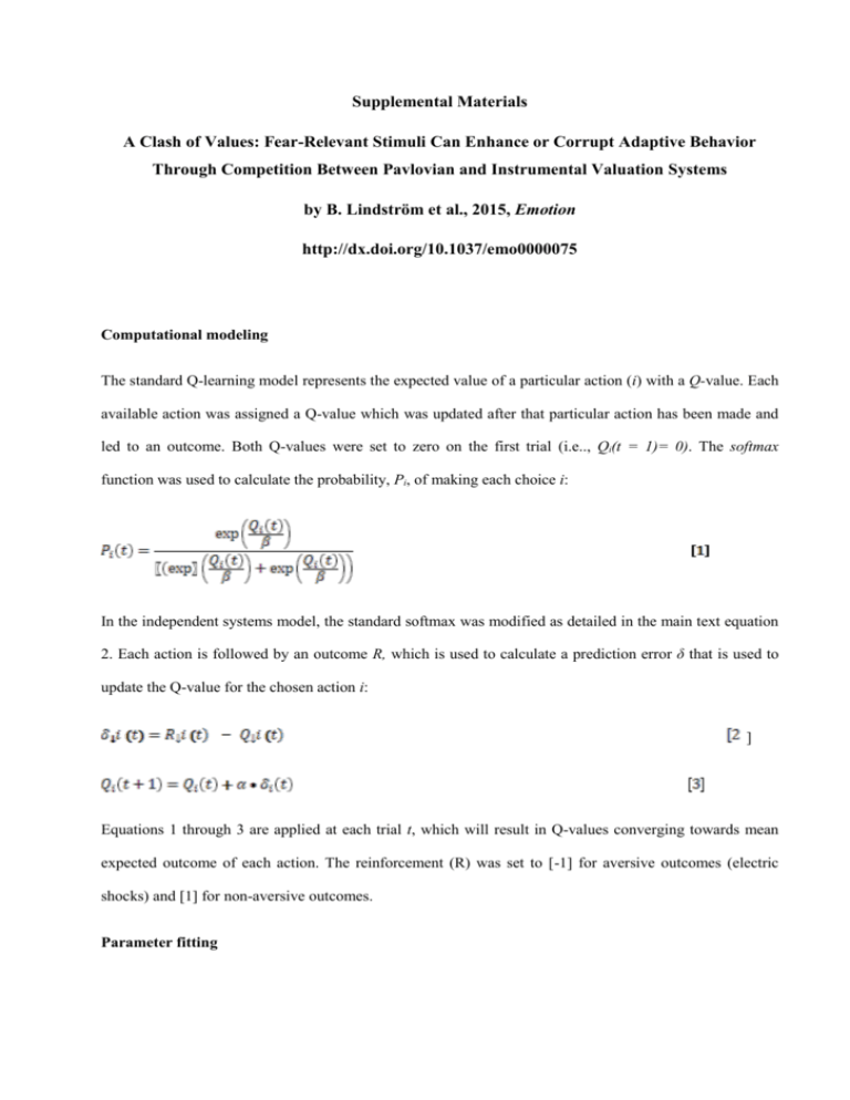
Supplemental Materials
A Clash of Values: Fear-Relevant Stimuli Can Enhance or Corrupt Adaptive Behavior
Through Competition Between Pavlovian and Instrumental Valuation Systems
by B. Lindström et al., 2015, Emotion
http://dx.doi.org/10.1037/emo0000075
Computational modeling
The standard Q-learning model represents the expected value of a particular action (i) with a Q-value. Each
available action was assigned a Q-value which was updated after that particular action has been made and
led to an outcome. Both Q-values were set to zero on the first trial (i.e.., Qi(t = 1)= 0). The softmax
function was used to calculate the probability, Pi, of making each choice i:
In the independent systems model, the standard softmax was modified as detailed in the main text equation
2. Each action is followed by an outcome R, which is used to calculate a prediction error δ that is used to
update the Q-value for the chosen action i:
]
Equations 1 through 3 are applied at each trial t, which will result in Q-values converging towards mean
expected outcome of each action. The reinforcement (R) was set to [-1] for aversive outcomes (electric
shocks) and [1] for non-aversive outcomes.
Parameter fitting
Parameter fitting was conducted using the maximum-likelihood approach, which finds the set of parameters
that maximize the probability of the participant´s trial-by-trial choices given the model. Optimization was
done by to minimizing the negative log-likelihood, -L, computed by:
where T denotes the total number of trials. Parameters were independently fitted to each subject using the
BFGS optimization method. Model implementations and parameter fitting was done in R (R Development
Core Team, 2012). All parameters were constrained to [0,1].
Model comparison
Model comparison was conducted using the Akaike Information Criterion (AIC), which measure the
goodness of fit of a model while also taking into account its complexity (Daw, 2011):
where k is the number of fitted parameters and –ln(L) is the negative log-likelihood. We used paired sample
t-tests of the AIC values to compare goodness of fit of the candidate models, thereby taking into account
individual differences in the model fits (see Methods).
Additional analysis of parameter estimates
In the main text, we analyzed the estimate Pavlovian parameter form the stimulus-bias model. We
also submitted estimated learning rate, α, to the same analysis. The average estimated α across the
experiments was relatively high (M = 0.52, SD = 0.35), as reflected in rapid asymptotic
performance, although with a high degree of between subjects variability (see Figure S1). There
was a significant effect of fear- type (F(3,149) = 3.28, p = 0.023), which reflected lower estimated
α for guns relative to out-group faces (regression simple effect estimate: β = -0.241, SE = 0.077, t
= -3.136, p = 0.002), but not any other type (ps > 0.084). Regression diagnostics revealed no
extreme outliers. Finally, the estimated β parameter was submitted to the same analysis, which
showed no main effect of Pavlovian trigger type (F(3,149) = 2.01, p = 0.11). Simple effects
showed that the estimated β was higher in the gun experiment than in the snake experiment
(regression simple effect estimate: β = 0.176, SE = 0.081, t = 2.178, p = 0.031), but was otherwise
comparable across experiments (ps > .05). Again, there were no extreme outliers. Neither the
estimated α parameter, nor the β parameter correlated significantly with the measures of individual
differences in racial bias or snake fear (ps > .1).
Alternative models
No bias
The No bias model was an unmodified Rescorla-Wagner model:
Changing bias
To determine the flexibility of the Pavlovian influence on behavior, we considered a model where
it was updated as a function of the outcomes of choosing the Pavlovian trigger. The model was
implemented according to equations 1-2, with the following addition; an additional Pavlovianchange
parameter regulated the effective Pavlovian influence based on the learning history. The
Pavlovianchange parameter is similar to the learning rate in the standard Q-learning algorithm.
resulting in an decrease of the influence following a positive outcome (R = 1) and an increase of
the influence following a negative outcome (R = -1). The softmax function thus change to
Learning-bias 1:
We considered a learning-bias model where the learning rate for fear-relevant stimuli differed as a function
of the outcome of the choice.
Learning-bias 2:
We also considered a model with different learning-rates for neutral and fear-relevant stimuli regardless of
the outcome of choices, reflecting possible differences in stimulus salience.
where
is the learning rate determining how much the prediction error will affect the
subsequent expected value of choosing the fear-relevant stimulus, and
is the learning
rate associated with neutral stimuli.
References.
Daw, N. D. (2011). Trial-by-trial data analysis using computational models. In M. R. Delgado, E. Phelps,
& T. W. Robbins (Eds.), Decision Making, Affect, and Learning: Attention and Performance XXIII
(pp. 1–26). New York: Oxford University Press.