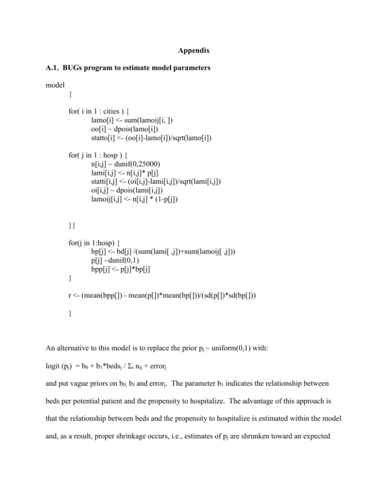
Appendix
A.1. BUGs program to estimate model parameters
model
{
for( i in 1 : cities ) {
lamo[i] <- sum(lamoij[i, ])
oo[i] ~ dpois(lamo[i])
statto[i] <- (oo[i]-lamo[i])/sqrt(lamo[i])
for( j in 1 : hosp ) {
n[i,j] ~ dunif(0,25000)
lami[i,j] <- n[i,j]* p[j]
statti[i,j] <- (oi[i,j]-lami[i,j])/sqrt(lami[i,j])
oi[i,j] ~ dpois(lami[i,j])
lamoij[i,j] <- n[i,j] * (1-p[j])
}}
for(j in 1:hosp) {
bp[j] <- bd[j] /(sum(lami[ ,j])+sum(lamoij[ ,j]))
p[j] ~dunif(0,1)
bpp[j] <- p[j]*bp[j]
}
r <- (mean(bpp[]) - mean(p[])*mean(bp[]))/(sd(p[])*sd(bp[]))
}
An alternative to this model is to replace the prior pj ~ uniform(0,1) with:
logit (pj) = b0 + b1*bedsj / i nij + errorj
and put vague priors on b0, b1 and errorj. The parameter b1 indicates the relationship between
beds per potential patient and the propensity to hospitalize. The advantage of this approach is
that the relationship between beds and the propensity to hospitalize is estimated within the model
and, as a result, proper shrinkage occurs, i.e., estimates of pj are shrunken toward an expected
value based on the number of beds per potential patient. This model might indicate a stronger
relationship between the number of beds and the propensity to hospitalize than the one we find.
The problem is that estimating the posterior distribution for the parameters of this modified
model is not easily implemented with the usual Gibbs sampling approaches used in BUGS since
unknown parameters must be jointly randomized. For computational simplicity, we opted to use
the model in the program.
A.2. BUGs program to simulate data and test alternative estimates
model
{
for( i in 1 : 70) {
lamo[i] <- sum(lamoij[i, ])
oo[i] ~ dpois(lamo[i])
for( j in 1 : 66 ) {
n[i,j] ~ dunif(100,1000)
lami[i,j] <- n[i,j]* p[j]
oi[i,j] ~ dpois(lami[i,j])
lamoij[i,j] <- n[i,j] * (1-p[j])
}}
for(j in 1:66) {
bp[j] <- bd[j] /(sum(lami[ ,j])+sum(lamoij[ ,j]))
p[j] ~dunif(0,1)
bpf[j] <- p[j]*bp[j]
}
for(i in 1:70) {
for(j in 1:66) {
allocb[i,j] <- bd[j]*(oi[i,j]/(sum(oi[ ,j])))
# allocb[i,j] are beds from hospital j allocated to area i
}
o[i] <- sum(oi[i, ])
allocbi[i] <- sum(allocb[i, ])
oall[i] <- o[i]*allocbi[i]
prin[i] <- sum(oi[i, ]) /(sum(oi[i,])+sum(oo[i]))
prinpall[i] <- prin[i]*allocbi[i]
}
bugsr <- (mean(bpp[]) - mean(p[])*mean(bp[]))/(sd(p[])*sd(bp[]))
approxbr <- (mean(prinpall[]) –
mean(prin[])*mean(allocbi[]))/(sd(prin[])*sd(allocbi[]))
diffr <- abs(bugsr-approxbr)
wennr <- (mean(oall[]) –
mean(o[])*mean(allocbi[]))/(sd(o[])*sd(allocbi[]))
A.3. Example to show that the non-Bayesian bed-allocation method does not induce a
correlation between beds and hospitalizations.
In this example, we consider two areas, each of which has a population of 100 people, and two
hospitals, each of which has one bed. In addition to the 2 areas of interest, each hospital serves a
number of other areas, which we combine into a category “all other areas” and denote by AOA.
In the example that follows, we show that, as a result of the way in which beds are allocated to
areas, the traditional method of analysis will always find support for Roemer’s Law. The nonBayesian bed allocation method, which uses the same bed allocation method as the traditional
approach, does not necessarily find support for Roemer’s Law.
Table 1: Number of inpatients at Hospital j from Area i (Iij) and number of outpatient-only
patients in Area i (Oi)
Area 1
Area 2
AOA
Hospital 1
5
0
5
Hospital 2
0
6
5
Outpatients-only
15
varies: 14, 16, 18
0
Table 2: Allocated beds from Hospital j to Area i (= (Iij / i Iij)*(bedsj))
Area 1
Area 2
AOA
Hospital 1
(5/10)*1 = .5
0
(5/10)*1 = .5
Hospital 2
0
(6/11)*1 = .5455
(5/11)*1 = .4545
Traditional method: The traditional method compares allocated beds per person to inpatients per
person. The number of outpatients in an area is not considered. Table 3 shows the data for this
analysis.
Table 3: Allocated beds per person and inpatients per person
Area 1
Area 2
Allocated beds per person
.5/100
= .005
.5455/100 = .005455
Inpatients per person
5/100 = .05
6/100 = .06
The correlation of allocated beds per person and inpatients per person for these two data points is
positive: more beds per person are associated with more inpatients per person, a finding
consistent with Roemer’s Law.
Non-Bayesian bed allocation method: This method compares allocated beds per potential patient
to inpatients per potential patient. Potential patients are inpatients plus those treated as
outpatients-only.
Table 4: Allocated beds per potential patient and inpatients per potential patient
Area 1: O1 = 15
Allocated beds per potential patient:
Inpatients per potential patient:
Area 2: O2 = 14
Allocated beds per potential patient:
Inpatients per potential patient:
Area 2: O2 = 16
Allocated beds per potential patient:
Inpatients per potential patient:
Area 2: O2 = 18
Allocated beds per potential patient:
Inpatients per potential patient:
.5/20
5/20
= .0250
= .2500
.5455/20
6/20
= .0273
= .3000
.5455/22
6/22
= .0248
= .2730
.5455/24
6/24
= .0227
= .2500
For the two data points (area 1 and area 2), the correlation of allocated beds per potential patient
and inpatients per potential patient is as follows: 1) positive when O2 =14, a finding consistent
with Roemer’s Law (since when more beds are available, the hospitalization rate is higher); 2)
negative when O2 =16, a finding the opposite of Roemer’s Law (since when fewer beds are
available, the hospitalization rate is higher); and 3) cannot be calculated when O2 =18 since there
is no variation in one of the variables.
Conclusion: This example shows the traditional method used to analyze Roemer’s Law induces
a positive correlation between beds and hospitalizations in an area. Our non-Bayesian bed
allocation method does not induce a positive correlation. The correlation could be positive,
negative, or un-calculable depending on the ratio of inpatients to outpatients.