The Carbon Cycle – Analyzing Atmospheric Data
advertisement
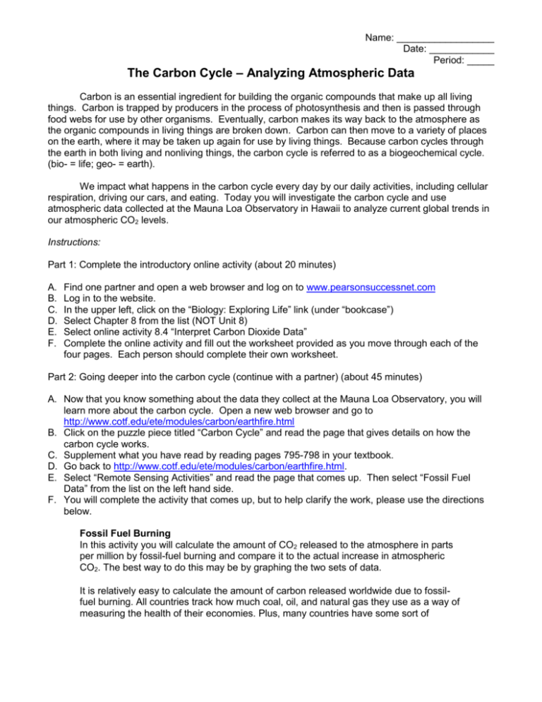
Name: __________________ Date: ____________ Period: _____ The Carbon Cycle – Analyzing Atmospheric Data Carbon is an essential ingredient for building the organic compounds that make up all living things. Carbon is trapped by producers in the process of photosynthesis and then is passed through food webs for use by other organisms. Eventually, carbon makes its way back to the atmosphere as the organic compounds in living things are broken down. Carbon can then move to a variety of places on the earth, where it may be taken up again for use by living things. Because carbon cycles through the earth in both living and nonliving things, the carbon cycle is referred to as a biogeochemical cycle. (bio- = life; geo- = earth). We impact what happens in the carbon cycle every day by our daily activities, including cellular respiration, driving our cars, and eating. Today you will investigate the carbon cycle and use atmospheric data collected at the Mauna Loa Observatory in Hawaii to analyze current global trends in our atmospheric CO2 levels. Instructions: Part 1: Complete the introductory online activity (about 20 minutes) A. B. C. D. E. F. Find one partner and open a web browser and log on to www.pearsonsuccessnet.com Log in to the website. In the upper left, click on the “Biology: Exploring Life” link (under “bookcase”) Select Chapter 8 from the list (NOT Unit 8) Select online activity 8.4 “Interpret Carbon Dioxide Data” Complete the online activity and fill out the worksheet provided as you move through each of the four pages. Each person should complete their own worksheet. Part 2: Going deeper into the carbon cycle (continue with a partner) (about 45 minutes) A. Now that you know something about the data they collect at the Mauna Loa Observatory, you will learn more about the carbon cycle. Open a new web browser and go to http://www.cotf.edu/ete/modules/carbon/earthfire.html B. Click on the puzzle piece titled “Carbon Cycle” and read the page that gives details on how the carbon cycle works. C. Supplement what you have read by reading pages 795-798 in your textbook. D. Go back to http://www.cotf.edu/ete/modules/carbon/earthfire.html. E. Select “Remote Sensing Activities” and read the page that comes up. Then select “Fossil Fuel Data” from the list on the left hand side. F. You will complete the activity that comes up, but to help clarify the work, please use the directions below. Fossil Fuel Burning In this activity you will calculate the amount of CO2 released to the atmosphere in parts per million by fossil-fuel burning and compare it to the actual increase in atmospheric CO2. The best way to do this may be by graphing the two sets of data. It is relatively easy to calculate the amount of carbon released worldwide due to fossilfuel burning. All countries track how much coal, oil, and natural gas they use as a way of measuring the health of their economies. Plus, many countries have some sort of environmental protection agency which tracks emissions. So how many tons of CO2 are released to the atmosphere from fossil-fuel burning is fairly accurately known. 1. Download the Excel spreadsheet file indusco2.xls. This is found under #1 on the “Fossil Fuel Burning page. Select all of the data in the spreadsheet, then copy and paste it all into a new excel spreadsheet. This file contains the total emissions from fossil-fuel burning in million metric tons of carbon for each year since 1959. 2. Using the data in the total column, calculate how much CO2 in parts per million was released to the atmosphere each year. There are instructions on how to do this if you click on the link in step 2 of the directions on the computer. Remember that your data is given in millions of metric tons of C. Your data from this step should be put in a new column that has been labeled “calculated ppm of C”. This shows how much C was added to the atmosphere each year. (You may need to use multiple columns to get the math done, just follow the steps on the website.) NOTE: all of your values should fall between 1 – 3 ppm. NOTE ON SIMPLIFYING CALCULATIONS: If you want to do a similar calculation for a whole column in excel, type in the calculation in the first box and press Enter. Then click on that box and press copy. Then highlight all of the boxes that this calculation applies to and press paste. After this is done, click on a few of the resulting values, double check that the correct equation was used and make sure they seem reasonable. (If you are stuck, ask another group for help with this.) 3. Calculate the total cumulative amount of C in the atmosphere each year. First, title a new column “calculated cumulative ppm of C”. The level of C in the atmosphere at the end of 1958 was 314.5 ppm, so to find out the calculated cumulative C level for 1959, add 314.5ppm to the total amount released in 1959 (found in the “calculated ppm of C” column). To find the value for 1960, add the number you just found to the total amount released in 1960. Continue this for each year on the spreadsheet. These numbers tell you the calculated levels of CO2 for each year assuming no CO2 was removed from the atmosphere. 4. Now you can compare your calculated ppm of C for each year with the actual C levels that were taken from the Mauna Loa observatory. To get these, click on the “Mauna Loa Data Set” under #4 on the Fossil Fuel Burning web page. A spreadsheet showing monthly and total C readings will come up. Highlight the column on the right hand side titled “Annual” and paste it into your excel spreadsheet next to your calculated cumulative C levels. 5. Construct a graph that compares the amount of C in the atmosphere that was expected and that was actually found. Your graph should have Years listed on the x axis and levels of C (ppm) on the y axis. You should graph two curves on the same page, one showing the “calculated cumulative ppm of C” and the other showing the annual measurements taken from the observatory. Adjust the scale on both axes so that your graph is clearly visible, taking up most of the graph page. 6. Write a paragraph comparing the two curves you have made. In your paragraph, account for any differences you see between the expected and the actual C values. 7. Print out a copy of your excel spreadsheet, your graph, and your paragraph. Write both of your names on it, staple it, and hand it in to the sub. Part 3: The Kyoto Protocol vs. Bush’s Clear Skies Plan (about 30 minutes) The world is concerned about rising atmospheric CO2 levels because they can lead to a variety of environmental issues, including global warming. Many countries, including in the world, including the US, have signed on to an agreement called the Kyoto Protocol whose main goal is to reduce CO2 emissions. Shortly after signing the Kyoto Protocol, President George W. Bush instituted a separate program called the Clear Skies Plan to help reduce emissions. This angered many people because it seemed to sidestep the Kyoto Protocol that we had previously signed. Using the internet, research the Kyoto Protocol and Bush’s Clear Skies Plan and find out what the differences are between them. Then, with your partner on google docs, compare and contrast the two plans and explain why so many people are upset about them. If you do not have time to complete this in class, do it independently for homework.
