Excerpted from
http://www.csie.ndhu.edu.tw/~rschang/chap7.doc:
 Linear programming with two variables

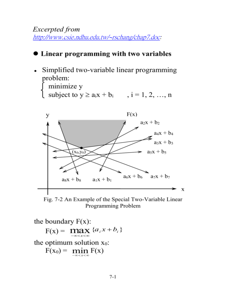
Simplified two-variable linear programming
problem:
minimize y
subject to y  aix + bi
, i = 1, 2, …, n
F(x)
y
a2x + b2
a4x + b4
a3x + b3
a5x + b5
(x0,y0)
a8x + b8
a1x + b1
a6x + b6
a7x + b7
x
Fig. 7-2 An Example of the Special Two-Variable Linear
Programming Problem
the boundary F(x):
{a i x  bi }
F(x) = max
  x  
the optimum solution x0:
F(x0) = min
F(x)
 x
7-1
Delete constraints:
y
a1x + b1
a2x + b2
a4x + b4
a3x + b3
a5x + b5
May be deleted
a6x + b6
a8x + b8
a7x + b7
x0
x
xm
Fig. 7-3 Constraints which May be Eliminate in the
Two-Variable Linear Programming Problem
If x0 < xm and the intersection of a1x + b1 and a2x +
b2 is greater than xm, then one of these two
constraints is always smaller than the other for x <
xm. Thus, this constraint can be deleted.
It is similar for x0 > xm.
7-2

Suppose an xm is known. How do we know
whether x0 < xm or x0 > xm ?
Let ym = F(xm) =
max {a x
i
1 i  n
m
 bi }
Case 1: ym is on only one constraint.
y
y'm
x0
x0
x0
ym
x'm
xm
x
Fig.7-5 The Cases where xm Is on Only One Constrain
Let g denote the slope of this constraint.
If g > 0, then x0 < xm.
If g < 0, then x0 > xm.
7-3
Case 2: ym is the intersection of several constraints.
y
gmin
gmax
gmin
gmax
gmin
gmax
Case 2a: xm,3
Case 2b: xm,1
Case 2c: xm,2
x
xm,1
xm,2
xm,3
Fig. 7-6 Cases of xm on the Intersection of Several Constraints
Let gmax =
max{a
slope
gmin =
min {a
1i  n
1 i  n
i
i
| ai xm  bi  F ( xm )} , max.
| ai x m  bi  F ( x m )} , min. slop
Case 2a: gmin > 0, gmax > 0  x0 < xm
Case 2b: gmin < 0, gmax < 0  x0 > xm
Case 2c: gmin < 0, gmax > 0  (xm, ym) is the
optimum solution.

How do we choose xm ?
We arbitrarily group the n constraints into n/2
pairs. For each pair, find their intersection.
Among these n/2 intersections, choose the
median of their x-coordinates as xm.
7-4
Algorithm 7.2 A Prune-and-Search Algorithm
to Solve a Special Linear Programming
Problem.
Input: Constrains S: ajx + bj, i=1, 2, …, n.
Output: The value x0 such that y is minimized at
x0 subject to y  ajx + bj, i=1, 2, …, n.
Step 1. If S contains no more than two constraints,
solve this problem by a brute force method.
Step 2. Divide S into n/2 pairs of constraints. For
each pair of constraints aix + bi and ajx + bj,
find the intersection pij of them and denote
its x-value as xij.
Step 3. Among the xij’s (at most n/2) of them , find
the median xm.
{ai xm  bi }
Step 4. Determine ym = F(xm) = max
1 i  n
gmin =
gmax =
min {a | a x  b  F ( x )}
max{a | a x  b  F ( x )}
1i  n
1 i  n
i
i
i
m
i
m
i
m
i
m
Step 5.
Case 5a. If gmin and gmax are not of the same
sign, ym is the solution and exit.
Case 5b. otherwise, x0 < xm, if gmin > 0, and x0
>xm, if gmin < 0.
Step 6.
Case 6a. If x0 < xm, for each pair of constraints
whose x-coordinate intersection is
7-5
larger than xm, prune away the
constraint which is always smaller
than the other for x  xm.
Case 6b. If x0 > xm, for each pair of constraints
whose x-coordinate intersection is less
than xm, prune away the constraint
which is always smaller than the other
for x xm.
Let S denote the remaining of contains. Go to
Step 2.
There are totally n/2 intersections. Thus, n/4
constraints are pruned away for each iteration.
time complexity: O(n)
7-6
 The
general
two-variable
programming problem:
linear
minimize ax + by
subject to aix + biy  ci , i = 1, 2, …, n
Let x’ = x
y’ = ax + by

minimize y’
subject to ai’x’ + bi’y’  ci’ , i = 1, 2, …, n
where ai’ = ai –bia/b
bi’ = bi/b
ci’ = ci
Change the symbols and rewrite as:
minimize y
subject to y  aix + biy ( i  I1 )
y  aix + biy ( i  I2 )
axb
7-7
define:
F1(x) = max {aix + bi , i  I1}
F2(x) = min {aix + bi , i  I2}
y
F2(x)
F1(x)
a
b

minimize F1(x)
subject to F1(x)  F2(x)
axb
7-8
x
a3x + b3
y
a5x + b5
a1x + b1
a4x + b4
a2x + b2
X
xm
x0
Fig. 7-9 The Pruning of Constraints for the General
Two-Variable Linear Programming Problem
In Fig. 7-9, if we know x0 < xm , then a1x + b1 can
be delete because a1x + b1 < a2x + b2 for x< xm.
Let F(x) = F1(x) - F2(x)
xm is feasible  F(xm)  0
define:
gmin = min {ai | i  I1, aixm + bi = F1(xm)},
min. slope
gmax = max{ai | i  I1, aixm + bi = F1(xm)},
max. slope
hmin = min {ai | i  I2, aixm + bi = F2(xm)},
min. slope
hmin = max{ai | i  I2, aixm + bi = F2(xm)},
max. slope
7-9
Case 1: F(xm)  0
 xm is feasible
(a) If gmin > 0, gmax > 0, then x0 < xm.
y
F2(x)
gmax
F1(x)
gmin
x
x0  xm
(b) If gmin < 0, gmax < 0, then x0 > xm.
y
F2(x)
F1(x)
gmin
xm x0
7-10
gmax
x
(c) If gmin < 0, gmax > 0, then xm is the optimum
solution.
y
F2(x)
F1(x)
gmin
gmax
x
xm = x0
Case 2: F(xm) > 0
 xm is infeasible
(a) If gmin > hmax, then x0 < xm.
y
F1(x)
gmin
hmax
F2(x)
x0 xm
7-11
x
(b) If gmin < hmax, then x0 > xm.
y
F1(x)
gmax
hmin
F2(x)
x
xm  x0
(c) If gmin  hmax, and gmax  hmin, then no
feasible solution exists.
y
F1(x)
gmax
gmin
hmax
hmin
F2(x)
x
xm
7-12
Algorithm 7.3 A Prune-and-Search Algorithm
to Solve the Two-Variable Linear Programming
Problem.
Input: I1: y  aix + bi, i = 1, 2, …, n1
I2: y  aix + bi, i = n1+1, n1+2, …, n.
axb
Output: The value x0 such that
y is minimized at x0
subject to y  aix + bi, i = 1, 2, …, n1
y  aix + bi, i = n1+1, n1+2, …, n.
axb
Step 1. Arrange the constraints in I1 and I2 into
arbitrary disjoint pairs respectively. For
each pair, if aix + bi is parallel to ajx + bj,
delete aix + bi if bi < bj for i, jI1 or bi > bj
for i, jI2. Otherwise, find the intersection
pij of y = aix + bi and y = ajx + bj. Let the
x-coordinate of pij be xij.
Step 2. Find the median xm of xij’s (at most  n2  of
 
them).
Step 3. (a) If xm is optimal, report this and exit.
(b) If no feasible solution exists, report this
and exit.
(c)Otherwise, determine whether the
optimum solution lies to the left, or right,
of xm.
7-13
Step 4. Discard at least 1/4 of the constraints.
Go to Step 1.
time complexity: O(n)
7-14