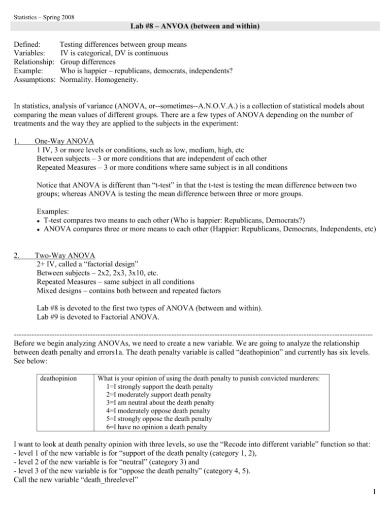
Statistics – Spring 2008
Lab #8 – ANVOA (between and within)
Defined:
Variables:
Relationship:
Example:
Assumptions:
Testing differences between group means
IV is categorical, DV is continuous
Group differences
Who is happier – republicans, democrats, independents?
Normality. Homogeneity.
In statistics, analysis of variance (ANOVA, or--sometimes--A.N.O.V.A.) is a collection of statistical models about
comparing the mean values of different groups. There are a few types of ANOVA depending on the number of
treatments and the way they are applied to the subjects in the experiment:
1.
One-Way ANOVA
1 IV, 3 or more levels or conditions, such as low, medium, high, etc
Between subjects – 3 or more conditions that are independent of each other
Repeated Measures – 3 or more conditions where same subject is in all conditions
Notice that ANOVA is different than “t-test” in that the t-test is testing the mean difference between two
groups; whereas ANOVA is testing the mean difference between three or more groups.
Examples:
● T-test compares two means to each other (Who is happier: Republicans, Democrats?)
● ANOVA compares three or more means to each other (Happier: Republicans, Democrats, Independents, etc)
2.
Two-Way ANOVA
2+ IV, called a “factorial design”
Between subjects – 2x2, 2x3, 3x10, etc.
Repeated Measures – same subject in all conditions
Mixed designs – contains both between and repeated factors
Lab #8 is devoted to the first two types of ANOVA (between and within).
Lab #9 is devoted to Factorial ANOVA.
--------------------------------------------------------------------------------------------------------------------------------------------Before we begin analyzing ANOVAs, we need to create a new variable. We are going to analyze the relationship
between death penalty and errors1a. The death penalty variable is called “deathopinion” and currently has six levels.
See below:
deathopinion
What is your opinion of using the death penalty to punish convicted murderers:
1=I strongly support the death penalty
2=I moderately support death penalty
3=I am neutral about the death penalty
4=I moderately oppose death penalty
5=I strongly oppose the death penalty
6=I have no opinion a death penalty
I want to look at death penalty opinion with three levels, so use the “Recode into different variable” function so that:
- level 1 of the new variable is for “support of the death penalty (category 1, 2),
- level 2 of the new variable is for “neutral” (category 3) and
- level 3 of the new variable is for “oppose the death penalty” (category 4, 5).
Call the new variable “death_threelevel”
1
1. Graphing
 The first step of any statistical analysis is to first graphically plot the data.
 There are two types of graphical plots for ANOVA data.
a. The first type of graphical plot is provided by using the Graphs --> Legacy Dialogs --> Error Bars.
This type of plot provides confidence intervals which are useful when visually inspecting the data.
b. The second type of graphical plot is provided when you conduct the analysis (ANOVA), but the plot
does not include confidence intervals. As you become more experienced analyzing data, you will
realize that you don’t need to conduct the first type of graphical plot that contains the confidence
intervals because the same information is provided non-graphically in the output for each analysis.
 In this section I will explain how to conduct the first type of plot that contains confidence intervals.
 In later sections when I show you how to conduct ANOVAs, I will show you how to conduct the second type
of plot.
 How do How do I plot the data?
1. Select Graphs --> Legacy Dialogs --> Error Bars
2. Click “Simple”, and “Define”
3. Move the categorical variable (IV) into the “Category Axis” and move the DV into the “variable” box.
4. Click OK.
 The output below indicates that level 1 (support) and level 2 (neutral) are similar to each, and both are
different from level 3 (oppose). In other words, I would suspect that those subjects who oppose the death
penalty are significantly different on errors1a than subjects who support or are neutral toward the death
penalty. This makes sense conceptually because lower on errors1a indicates that you would rather acquit
guilty people than convict innocent people. In other words, opposing the death penalty is associated with
opposing to convict innocent people.
2. Assumptions - Homogeneity
 When dealing with group means (t-test, ANOVA), there are two assumptions: Normality and Homogeneity.
 Normality was discussed in Lab #1.
 Homogeneity is whether the variances in the populations are equal. When conducting an ANOVA, one of the
options is to produce a test of homogeneity in the output, called Levene’s Test.
a. If Levene’s test is significant (p < .05) then equal variances are NOT assumed, called heterogeneity.
b. If Levene’s is not significant (p > .05) then equal variances are assumed, called homogeneity.
 It doesn’t really matter whether you have homogeneity or heterogeneity since SPSS output gives you all
available information for both situations: equal variances assumed, and equal variances not assumed. See the
next section where I discuss the output generated by SPSS for t-tests.
 Levene’s Test is generated for both between ANOVAs and within ANOVAs
2
3. ANOVA between
 You conduct ANOVA between by:
1. Select Analyze --> Compare Means --> One-Way ANOVA
2. Move the DV into the “Dependent List” box, and move the IV into the “Factor” box.
3. Click “Post hoc” and click “LSD”
4. Click Options, and click “Descriptive” and “Homogeneity” and “Welch” and “Means plot”
4. Click OK.
 The output below is for “death_threelevels” and “errors1a”.
 The output is in four parts:
 Part 1 is the descriptive analysis. The second box tells you whether or not the data are homogeneous. Since
Levene’s test is significant, then equal variances are not assumed.

Part 2 is the Omnibus F. If Levene’s test from above is significant, then you use the data from the second box
which indicates the “Welch” test In this case, Levene’s test is significant (p = .026) so equal variances are not
assumed. The Omnibus F tells us if at least one of the pairwise comparisons is significant, but it does not
indicate which of the pairwise comparison(s) is significant. To find out which pairwise comparison is
significant, you need to do either Post-hocs or Planned Contrasts.

Part 3 are the multiple comparisons and plots. Some statistics books say that you can only test for Post-hoc
pairwise comparisons if the Omnibus F is significant, but other statistics books say you can test for Post-hoc
pairwise comparisons even if the Omnibus F is not significant. In this case, levels 1 (support) and 2 (neutral)
are significantly different than level 3 (oppose) but are not significantly different from each other.
FYI – I chose to use “LSD” as the post-hoc test. There are many different post-hoc options depending upon a
number of different factors. See the Field’s textbook 339 for how to make decisions about which post-hoc
option you want to use. I typically only use LSD because it is the least strict test.
3



The output provides information about significance value, but you have to calculate the effect size by hand.
The formula is on page 357 of Field’s textbook. The pieces of information required to calculate the effect size
are reported above in the output from SPSS – SS between and SS within. FYI – SS means “Sum of Squares”.
I haven’t found a website that will calculate the effect size for you. In this case the effect size is .195
WRITE-UP. The information included in the write up is the means, F value, df, and significance value. Lately,
the field as a whole has recommended that you report effect size as well.
a. The overall effect across conditions was significant, F(2, 119) = 6.705, p = .002. Post-hoc tests
indicated that participants who support the death penalty (M = 5.64) were significantly different than
participants who oppose the death penalty (M = 4.51), p = .002. Post-hoc tests also indicated that
participants who are neutral about the death penalty (M = 5.94) were significantly different than
participants who oppose the death penalty (M = 4.51), p = .004. The effect size is .195.
EVALUATION: Just like with evaluation all types of analyses involving group means (t-test, ANOVA), you
only really care about three pieces of information: (1) is the effect significant (p-value), (2) what is the size of
the effect (effect size), and (3) what is the direction of the effect (which mean is larger than the other).
4







Now, let’s do the same between ANOVA analysis, but this time use Planned Contrasts.
In the analysis above, we conducted Post-hoc tests. Another option is Planned Contrasts. Planned Contrasts
only test specific pairwise comparisons, as compared to Post-hoc tests which test all possible comparisons.
Planned Contrasts only tests specific chunks of variance, as compared to Omnibus F and post-hoc tests which
test all the variance.
You choose the specific Planned Contrasts based upon aprori hypotheses.
You conduct specific Planned Contrasts by using the “Contrast” option in SPSS. In essence, you assign
“weights” to the different pairwise comparisons. The rules for weighting Planned Contrasts are somewhat
complicated, so if you are thinking about conducting Planned Contrasts, start by reading page 325 of Field’s
textbook. Planned Contrasts are not as commonly conducted as Post-hoc tests, but I want to be aware of the
concept, so let’s do a concrete example using our dataset. Let’s say that we want to specifically test the
relationship between level 1 (support) and level 2 (neutral). You assign weights so that they sum to 0, and you
only assign weights to the levels you want to test. In this case, we would assign:
Level 1 = -1
Level 2 = 1
Level 3 = 0
Within SPSS you assign weights by:
1. Select Analyze --> Compare Means --> One-Way ANOVA
2. Move the DV into the “Dependent List” box, and move the IV into the “Factor” box.
3. Click “Contrasts” and click “polynomial”, and click degree that is “5th”
Then enter the coefficients one at a time. So -1, 1, 0.
4. Click Options, and click “Descriptive” and “Homogeneity” and “Welch” and “Means plot”
5. Click OK.
The output below is for “death_threelevels” and “errors1a”. Most of the output is the same as before when we
conducted the same analysis using Post-hoc tests, so below is only the output specific to Planned Contrasts.
a. ANOVA – Instead of reporting one Omnibus F, the output now displays an Omnibus F for Linear and
Quadratic situations. If our categorical variable has more levels (such as 4, 5, 6, etc) then even more
situations would appear in the output (such as cubic, 4th order, 5th order). You choose to report the
Omnibus F that corresponds to how your data are graphically represented. See the graphs on page 338
of Field’s textbook for graphically representations of the different situations.
b. Contrast Coefficients – This box reminds you how you weighted the levels
c. Contrast Tests – This box tells you if the specific Planned Contrast is significant. When conducting
Planned Contrasts you can divide the p-level by 2 to make the test “one-tailed”. I will explain about
“one-tailed” later, but for right now notice that it makes the p-level smaller, and thus closer to
significant. Thus, it is possible that you could find a non-significant relationship when analyzed as a
Post-hoc test, but find a significant relationship when analyzed as a Planned Comparison. For our
example, the significant is .479/2 = .24. This p-level is not significant.
5
4. ANOVA repeated
 We don’t have a repeated ANOVA factor in our dataset so we can’t use repeated ANOVA.
 However, imagine, just for the sake of argument, that system1, system2, and system3 are the same question.
Also imagine that we asked subjects to answer system1 before the study began, and that we asked subjects to
answer system2 in the middle of the study, and we asked subjects to answer system3 at the end of the study.
The hypothesis would be that answering questions about the legal system changed how subjects would answer
this question. For example, the hypothesis is that being exposed to the questions in the survey (such as flaws
in the legal system regarding convicting innocent people, problems with DNA evidence, etc) made the
subjects answer lower on the scale.
 How to conduct repeated ANOVA:
1. Select Analyze --> General Linear Model --> Repeated Measures
2. Enter the number of level into “Number of Levels”. In this case its “3”. Click “Add”. Click “Define”.
3. Move the three variables over to the “Within-Subjects” box.
4. Click “Plots”, move factor1 into the “Horizontal Axis” box, click “Add”, then “Continue”
5. Click “Options”, move “factor1” into the “Display Means” box, click “Compare Main Effects”.
FYI – this is the way you conduct Post-hoc analyses in repeated ANOVA
6. While still in “Options”, click “Descriptive”, “Effect Size”, click “Continue”
7. Click OK.
 I am going to explain the output in four separate parts.
 Part 1 is the descriptive statistics.
6

Part 2 is the Omnibus F. First you check the middle box to identify Sphericity, which is whether the variance
across conditions and across pairs is equal.
a. If the test is non-significant (p > .05), then sphericity exists. If sphericity exists, then look at the third
box where it says “Sphericity Assumed” to find the Omnibus F, which is p = .000
b. If the test is significant (p < .05), then sphericity does not exist. If Sphericity does not exist, you have
two options: (1) look at the Greenhouse-Geisser or Huynh-Feldt correction, or (2) look at the
Multivariate Tests box. The corrections correct for sphericity, whereas the Multivariate tests are not
based upon the assumption of sphericity. In all cases, the same result occurs, p = .000.
7

Part 3 are the post-hocs. You interpret the Post-hoc analysis just as you would for ANOVA between.

Part 4 is the graphical plot of the data:


The output provides information about effect size, called partial eta squared.
WRITE-UP. The information included in the write up is the means, F value, df, and significance value. Lately
the field as a whole has recommended that you report effect size as well. FYI – I am reporting results for
Greenhouse-Geisser). FYI – when all conditions are significantly different from each other, report the posthoc tests in a table.
a. The overall effect across conditions was significant, F(1.92, 621.44) = 208.62, p < .000. Post-hoc tests
indicated that all three conditions were significantly different from each other. The effect size is .392.
EVALUATION: Just like with evaluation all types of analysis involving group means (t-test, ANOVA), you
only really care about three pieces of information: (1) is the effect significant (p-value), (2) what is the size of
the effect (effect size), and (3) what is the direction of the effect (which mean is larger than the other).

8