1
Additional file 1 – Time Complexity Analysis
2
3
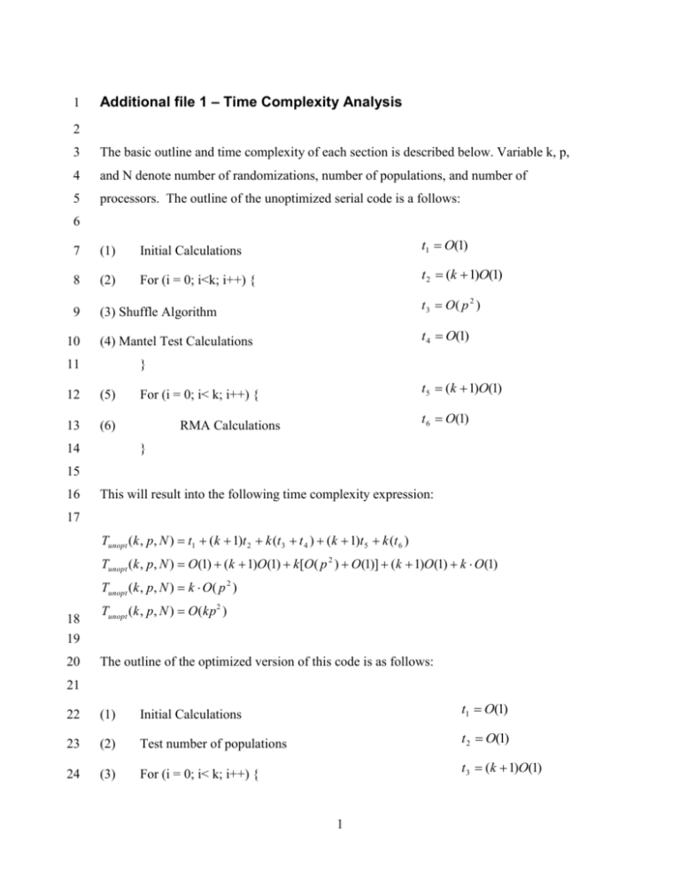
The basic outline and time complexity of each section is described below. Variable k, p,
4
and N denote number of randomizations, number of populations, and number of
5
processors. The outline of the unoptimized serial code is a follows:
6
7
(1)
Initial Calculations
t1  O(1)
8
(2)
For (i = 0; i<k; i++) {
t 2  (k  1)O(1)
9
(3) Shuffle Algorithm
t 3  O( p 2 )
(4) Mantel Test Calculations
t 4  O(1)
10
11
}
12
(5)
13
(6)
14
t 5  (k  1)O(1)
For (i = 0; i< k; i++) {
t 6  O(1)
RMA Calculations
}
15
16
This will result into the following time complexity expression:
17
Tunopt (k , p, N )  t1  (k  1)t 2  k (t 3  t 4 )  (k  1)t 5  k (t 6 )
Tunopt (k , p, N )  O(1)  (k  1)O(1)  k[O( p 2 )  O(1)]  (k  1)O(1)  k  O(1)
Tunopt (k , p, N )  k  O( p 2 )
18
19
20
Tunopt (k , p, N )  O(kp 2 )
The outline of the optimized version of this code is as follows:
21
22
(1)
Initial Calculations
t1  O(1)
23
(2)
Test number of populations
t 2  O(1)
24
(3)
For (i = 0; i< k; i++) {
t 3  (k  1)O(1)
1
25
(4) Optimized Shuffle Algorithm
t 4  O( p)
26
(5) Mantel Test Calculations
t 5  O(1)
27
t 6  O(1)
RMA Calculations
28
}
29
30
This leads into the following time complexity derivation for this code:
31
Topt (k , p, N )  t1  t 2  (k  1)t 2  k (t 4  t 5  t 6 )
Topt (k , p, N )  O(1)  O(1)  (k  1)O(1)  k[O( p)  O(1)  O(1)]
Topt (k , p, N )  k  O( p)
32
33
Topt (k , p, N )  O(kp)
34
Therefore, theoretical speedup of the optimized serial code verses the unoptimized serial
35
code is O(p):
SpeedupoptimizedVSunoptimized
36
O(kp2 )

 O( p )
Okp
.
37
This means that speedup should increase linearly with the number of populations. So, the
38
higher the population number, the more noticeable the speedup of the optimization.
39
40
Large populations in Figure 4 use the parallel version of the optimized code which is
41
outlined in the following:
42
43
(1)
Initial Calculations
t1  O(1)
44
(2)
Test number of populations
t 2  O(1)
45
(3)
Print data to file
t 3  O( p )
46
(4)
Start MPI multiple node processing
t 4  O( N )
(5)
k
For (i = 0; i< slice = N ; i++) {
k

t 5    1O(1)
N

47
2
48
(6)
Optimized Shuffle Algorithm
t 6  O( p )
49
(7)
Mantel Test Calculations
t 7  O(1)
50
(8)
RMA Calculations
t8  O(1)
51
52
}
The time complexity upper bound of the parallel code can be derived by the following:
53
54
55
k
k

T parallel (k , p, N )  t1  t 2  t 3  t 4    1O(1)  t 6  t 7  t 8 
N
N

k
T parallel (k , p, N )  O(1)  O( p)  O( N )   O( p )
N
k
T parallel (k , p, N )   O( p)
N
 kp 
T parallel (k , p, N )  O 
N
56
Therefore, theoretical speedup of the parallel code verses the unoptimized serial code is
57
O(pN):
Speedup parallelVSunoptimized
58
O(kp 2 )

 O( pN )
 kp 
O 
N
.
59
Here speedup is a factor of number of populations and the number of processors available
60
to the parallel code. Theoretical speedup of the parallel code verses the optimized serial
61
code is O(N):
Speedup parallelVSoptimized 
62
O(kp)
 O( N )
 kp 
O 
N
.
63
The theoretical speedup increases linearly with the number of processors available. This
64
increase is bounded by communication overhead (not included in above calculations)
65
which in the limit will eliminate the benefits if having more processors. Notice from the
66
figures when data are analyzed in parallel, they must be written to files. Files need to be
67
generated because the main code does not share memory with the parallel section. Values
68
are transferred by reading in data from files.
3