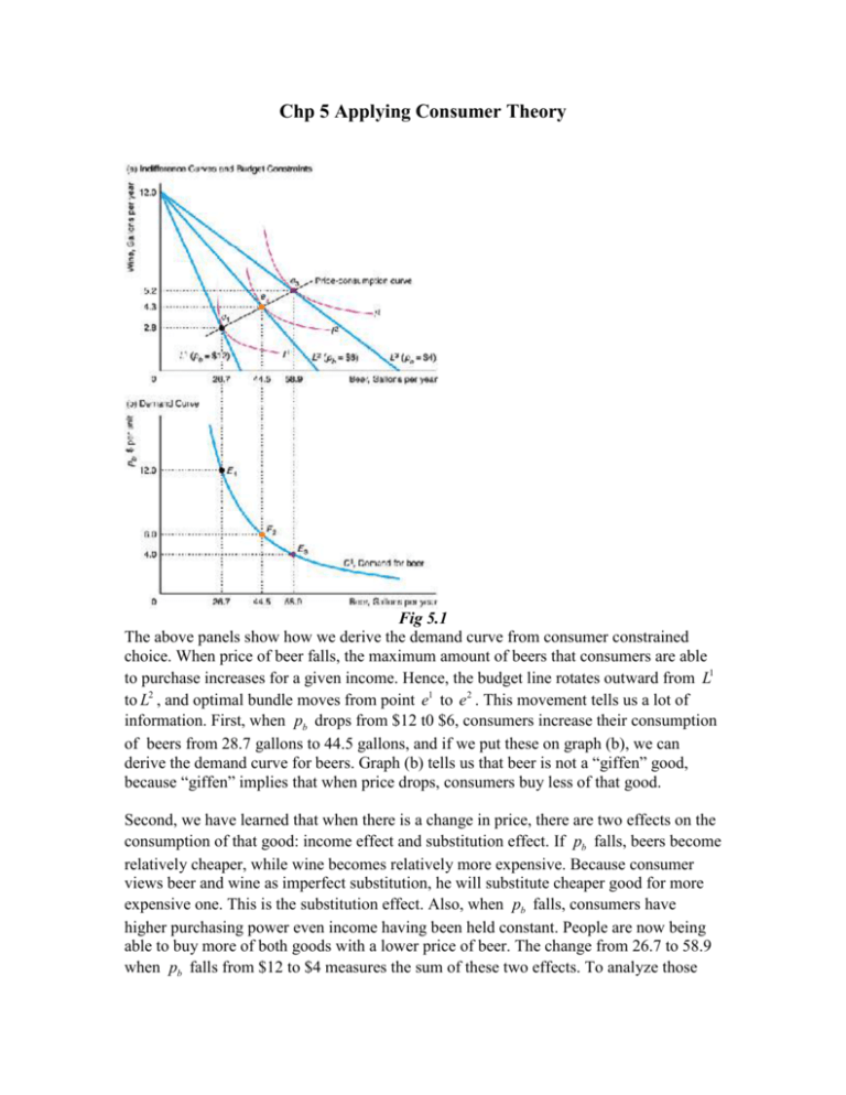
Chp 5 Applying Consumer Theory
Fig 5.1
The above panels show how we derive the demand curve from consumer constrained
choice. When price of beer falls, the maximum amount of beers that consumers are able
to purchase increases for a given income. Hence, the budget line rotates outward from L1
to L2 , and optimal bundle moves from point e1 to e 2 . This movement tells us a lot of
information. First, when pb drops from $12 t0 $6, consumers increase their consumption
of beers from 28.7 gallons to 44.5 gallons, and if we put these on graph (b), we can
derive the demand curve for beers. Graph (b) tells us that beer is not a “giffen” good,
because “giffen” implies that when price drops, consumers buy less of that good.
Second, we have learned that when there is a change in price, there are two effects on the
consumption of that good: income effect and substitution effect. If pb falls, beers become
relatively cheaper, while wine becomes relatively more expensive. Because consumer
views beer and wine as imperfect substitution, he will substitute cheaper good for more
expensive one. This is the substitution effect. Also, when pb falls, consumers have
higher purchasing power even income having been held constant. People are now being
able to buy more of both goods with a lower price of beer. The change from 26.7 to 58.9
when pb falls from $12 to $4 measures the sum of these two effects. To analyze those
two effects, we have to learn how to decompose the effect of a price change into income
effect and substitution effect.
Fig 5.2
Def of Substitution effect: If utility held constant, as the price of the good increases,
consumers substitute other, now relatively cheaper goods for that one.
Def of income effect: An increase in price reduces a consumer’s buying power,
effectively reducing the consumer’s income and causing the consumer to buy less of at
least some goods.
Suppose that we can take away some income from this consumer such that the budget
line will shift inward to L , an imaginary line tangent to I 1 . The tangent point is e . The
change from e1 to e in horizontal direction measures the substitution effect. Consumer
stays at the same utility level. However, with a relatively cheaper pb , the consumer will
increase his consumption of beer from 26.7 gallons to 30.6 gallons.
The shift from L to L2 shows an increase in the consumer’s income. His optimal bundle
moves from e to e2 , which measures the income effect on consumption of both goods.
The consumer now consumes 58.9 gallons of beer instead of 30.6 gallons.
SE  30.6  26.7  3.9
IE  58.9  30.6  28.3
 TE  SE  IE  32.2  58.9  26.7
The above example shows us how to decompose the effect of a price change into income
effect and substitution effect for a normal good. How do we know that is a normal good
case? From the income effect. A normal good says when the income increases, people are
going to buy more of that good, while less for an inferior good. So how do we decompose
for an inferior good?
The substitution effect is always the same. The only difference is the income effect.
Fig 5.3
This graph is a different example. Movie is an inferior good in this case. Price of movies
falls, and causes an outward rotation of the budget line. e1 to e still measures the
substitution effect. e to e2 measures the income effect. Since movie is an inferior good,
when income increases, the consumer actually goes less often to see the movies.
SE  (e  e1 ) M  0
IE  (e2  e ) M  0
TE  SE  IE  0 if | SE || IE | , i.e., SE dominates IE.
 0 if | SE || IE | , i.e., IE dominates SE (“Giffen” good).
“Giffen” good says when price of the good falls, people actually buy less of that good,
which also implies that the demand curve for the good is upward sloping.
Practice I: What would the value of the substitution effect be for two goods that are
perfect complements? Use a graph to demonstrate your answer.
Bonus (5pt): Sarah allocates her income of $5.00 between the consumption of donuts and
coffee. Her tastes and preferences are indicated by the indifference curves shown in
Figure 5.1. The price of donuts is $.50 each. Initially the price of coffee is $1.00 per cup.
Subsequently, the price of coffee falls to $.50 per cup. On the graph below, show the
initial utility maximizing position, the new utility maximizing position, and separate the
income and substitution effects. For Sarah, is coffee a normal or inferior good?
Deriving labor supply curve
Labor supply curve is the relationship between wage and quantity supplied of labor. From
the labor supply curve, we can tell how much one consumer is going to work for a given
wage. Most of supply curves come from producers’ side, i.e., firms’ side. However, since
labor supply is a decision made by consumers, we can apply consumer theory to derive
the labor supply curve.
So the question transforms to how much consumer want to consume the labor for every
given wage. But this question looks weird. Let’s put it this way: Everyone has a fixed
time endowment of 24 hours; among these 24 hours, people work and enjoy leisure.
Here, we denote all other kinds of activities except for work as leisure. Now, we can
rephrase the question: For a given wage, how much is the leisure demanded by
consumers?
We let N denote the time spent on leisure, H the time spent on working. Then we have
the following relationship: H  24  N .
Assume an individual has a preference: U (Y , N ) and his budget line is
Y  Y   wH  Y   w  24  N  , where Y  is any income other than labor-income. Y can
be thought of all other goods. Here, we let Y  be zero.
Fig 5.4
The intercept on x-axis means when consumer use all 24 hours on leisure, his income is
0, which implies he cannot consume any other goods. Intercept on y-axis means when he
works full time (24 hours), he achieves his maximum income at 24w , and his leisure is 0.
The slope of budget line is w . Note that wage w is viewed as the price of leisure. That
is because to get 1 unit of leisure, people have to give up 1 unit time of labor, i.e., income
of w .
If wage rate increases, intercept on x-axis does not change, while the intercept on y-axis
will be larger. Budget line rotates outward from L1 to L2 . Corresponding to the change of
the budget line, optimal consumption moves from e1 to e 2 . Initially, consumer is
enjoying 16 hours of leisure, while only works for 8 hours. But after the wage rate has
been increased, consumer now wishes to work more, 12 hours, and enjoy less of leisure,
12 hours also. So, if we put these on the demand curve for leisure, we can see it is a
downward sloping curve. And we can derive the supply curve of labor by the formula
H  24  N .
Fig 5.5
Now let’s decompose TE into IE and SE: (when leisure is a normal good)
Fig 5.6
SE: when w increases, leisure becomes more expensive, so consumers wish to work
more, enjoy less leisure. They are going to substitute labor for leisure. e1 to e measures
the SE.
IE: Wage increase causes income to increase, thus cause the shift of budget line from L
to L2 . Accordingly, optimal bundle moves from e to e 2 . Because leisure is a normal
good, consumer is going to increase his consumption of leisure.
SE: N  0 , IE: N  0
Commonly, TE=SE+IE>0, i.e., when wage increases, people decrease their consumption
of leisure, and work more.
Normally, when wage is quite low, leisure is viewed as an inferior good. And when wage
is sufficiently high, leisure becomes as a normal good.
Fig 5.7
Then we have this backward supply curve. When people start with a low wage, they want
to work to earn income so that they consume other goods. So for them, they would like to
work more when wage increases. However, when they become richer, they have had
enough wealth. Leisure becomes normal good. They want to enjoy leisure even wage is
quite high. So, when wage increases, they will supply less labor.