1.3 Expected Loss, Decision Rules, and Risk
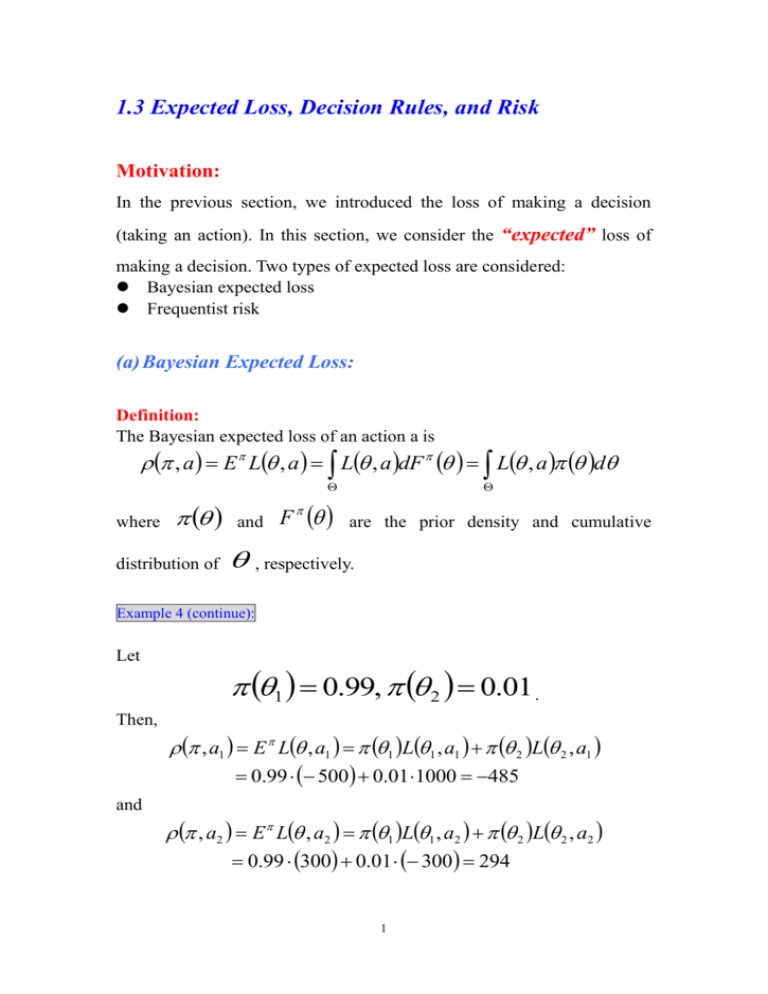
Motivation:
In the previous section, we introduced the loss of making a decision
(taking an action). In this section, we consider the “expected” loss of
making a decision. Two types of expected loss are considered:
 Bayesian expected loss
 Frequentist risk
(a) Bayesian Expected Loss:
Definition:
The Bayesian expected loss of an action a is
  , a   E  L , a    L , a dF      L , a   d

where
  
distribution of
and
F   

are the prior density and cumulative
 , respectively.
Example 4 (continue):
Let
 1   0.99,   2   0.01 .
Then,
  , a1   E  L , a1    1 L1 , a1     2 L 2 , a1 
 0.99   500  0.011000  485
and
  , a2   E  L , a2    1 L1 , a2     2 L 2 , a2 
 0.99  300  0.01   300  294
1
(b) Frequentist Risk:
Definition:
A (nonrandomized) decision rule
R
. If
 X 
is a function from  into
X  x0 is observed, then   x0  is the action that will be
taken. Two decision rules,
1
and
 2 , are considered equivalent if
P  1  X    2  X   1, for every  .
Definition:
The risk function of a decision rule
 X 
is defined by
R ,   E L ,  X    L , x dF X x |     L , x  f x |  dx

Definition:
If

R , 1   R ,  2 , for all    ,
 , then the decision rule 1
with strict inequality for some
R-better than the decision rule
is
 2 . A decision rule is admissible if
there exists no R-better decision rule. On the other hand, a decision rule
is inadmissible if there does exist an R-better decision rule.
Note:
A rule
1
is R-equivalent to
2
if
R , 1   R ,  2 , for all    .
2
Example 4 (continue):
R1 , a1   L1 , a1   500  300  L1 , a2   R1 , a2 
and
R 2 , a1   L 2 , a1   1000  300  L 2 , a2   R 2 , a2 .
Therefore, both
a1
and
a2
are admissible.
Example 5:
Let
X ~ N  ,1, L , a     a  ,  1  X   X ,  2  X  
2
Note that
E  X   
and
X
.
2
Var X   1.
Then,
R , 1   E L , 1  X   E L , X   E   X 
2
 Var  X   1
and
  X 
X

R ,  2   E L ,  2  X   E  L ,   E  

2 
2

 
X

X  
 E 
    E 
  
2 2
 2

 2
 X   2
  X   2
 E 
   2 
 

2
2  2
2
4 
 2
2
2
2
X 
X  
 E 
     E 
 
2
2
4
 2
 2
 2 Var ( X )  2
X
 Var    0 


4
4
4
 2
2
1 2
 
4
4
3
2
Definition:
The Bayes risk of a decision rule
on


with respect to a prior distribution
is defined as
r  ,    E  R ,     R , a   d

Example 5 (continue):
Let
 ~ N 0,  2 ,    
Then,
1
2  2
 2
e 2
r , 1   E  R , 1   E  1  1
and
1 2 

r  ,  2   E R ,  2   E  
4 4 
1 E  2
1 Var ( )
 
 
4
4
4
4
1 2
 
4
4


 
4
2