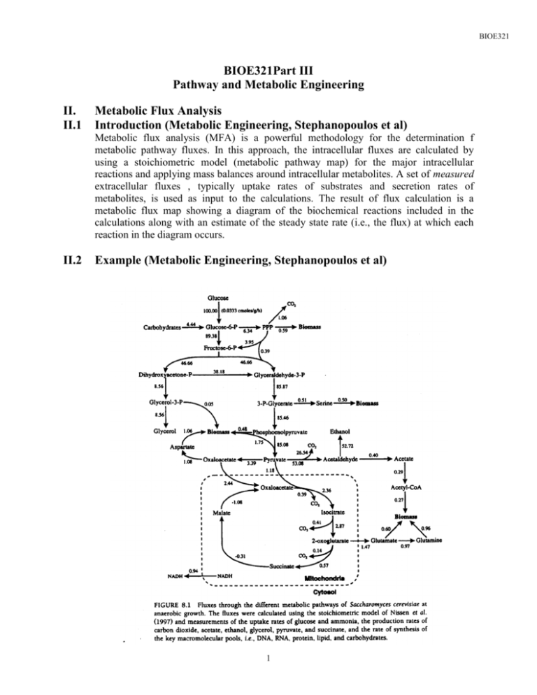
BIOE321
BIOE321Part III
Pathway and Metabolic Engineering
II.
II.1
Metabolic Flux Analysis
Introduction (Metabolic Engineering, Stephanopoulos et al)
Metabolic flux analysis (MFA) is a powerful methodology for the determination f
metabolic pathway fluxes. In this approach, the intracellular fluxes are calculated by
using a stoichiometric model (metabolic pathway map) for the major intracellular
reactions and applying mass balances around intracellular metabolites. A set of measured
extracellular fluxes , typically uptake rates of substrates and secretion rates of
metabolites, is used as input to the calculations. The result of flux calculation is a
metabolic flux map showing a diagram of the biochemical reactions included in the
calculations along with an estimate of the steady state rate (i.e., the flux) at which each
reaction in the diagram occurs.
II.2
Example (Metabolic Engineering, Stephanopoulos et al)
1
BIOE321
II.3
Other Applications of MFA
(Metabolic Engineering, Stephanopoulos et al)
2
BIOE321
II.3 Concept of reaction stoichiometry
Example 1
Consider a simple reaction network occurring in a constant volume cell shown in the
following diagram
So
r0
S
r1
r2
B
A
r3
r4
C
D
3
BIOE321
in the above reaction network, S0 is changed into S (this may consider as the intake of substrate
from outside of the cell), S is converted to A and B through reaction r1 and r2, A is converted to
C by reaction r3, and B is converted to D through reaction r4. Notice that in general the reaction
does not contain the stoichiometric information. It is usually accompanied by a set of
biochemical reactions, whose stoichiometric relationships have already established. For example,
Glucose + PEP -> Glucose-6-P + pyruvate
or
pyruvate + NADH -> lactate + NAD+
or
Glucose-6-P + ATP -> 2 Glyceraldehyde 3-P + ADP
Referring back to our previous example, suppose the reaction network follows the following
reactions
Referring back to our current example, suppose the reaction network follows the following
reactions
Reaction 0 :
0 S
So r

Reaction 1 :
r1 A
S 
2 B
S r

Reaction 2 :
3 C
A r
4 D
B r

Reaction 3 :
Reaction 4 :
Material Balance on the four species So, S, A, B and P, we have
dSo

dt
dS
dt
dA
dt
dB
dt
dC
dt
dD
dt
 ro

ro
 r1


r1

r3

r3

r4

r3

r4
r2
4
BIOE321
where ri is the reaction rate in proper units (such as mM/g-cell-hr). Or in a compact form we
have
SO 
S
 
d  A
 
dt  B 
C 
 
D 

0
0
0
 1 0
 rO 
 1 1 1 0
0  

 r1
1
0  1 0  
0

  r2 
0
0
1
0

1

 r 
3
0
0
0
1
0  

  r4 
0
0
0
1  
0
or
d ~
x
dt
~
 G T v~
where
~
x

SO 
S
 
 A
 
B
C 
 
D 
~
GT

0
0
0
 1 0
 1 1 1 0
0


1
0 1 0 
0


0
1
0  1
0
0
0
0
1
0


0
0
0
1
0
v~

 rO 
r 
 1
 r2 
 
 r3 
 r4 
x is commonly known as the state vector, which contains the state variables (in this case the
concentration of each of the species), GT is the stoichiometric matrix, and v is the reaction rector.
Note: the transpose of G is used as a symbol here because in some textbooks the state and
reaction vectors are a row vectors rather than a column vectors.
Question 1: The above formulation assumes the cell volume is constant, what
should be done if this assumption is to be removed? Or under what condition this
assumption is valid?
Question 2: how will the formulation of the problem change if
1 0.2 A
Reaction 1 :
S r
2  0.5B
Reaction 2 :
S r

5
BIOE321
Example 2
Consider another reaction network shown in the following schematic diagram
So
r0
S
r1
A
r2
r3
r4
B
P
in the above reaction network, S0 is changed into S (this may consider as the intake of substrate
from outside of the cell), S is converted to A and B through reaction r1 and r2, A is also
converted to B by reaction r3, finally, P is being formed from B through reaction r4. Notice that
as in the previous case, in general the reaction does not contain the stoichiometric information. It
is usually accompanied by a set of biochemical reactions, whose stoichiometric relationships
have already established. For example,
Glucose + PEP -> Glucose-6-P + pyruvate
or
pyruvate + NADH -> lactate + NAD+
or
Glucose-6-P + ATP -> 2 Glyceraldehyde 3-P + ADP
Referring back to our current example, suppose the reaction network follows the following
reactions
6
BIOE321
Reaction 0 :
0 S
So r

Reaction 1 :
1 0.5 A
S r
2  0.6B
S r

Reaction 2 :
3 0.8B
A r

4  0.7 P
B r

Reaction 3 :
Reaction 4 :
Material Balance on the four species So, S, A, B and P, we have
dSo

dt
dS
dt
dA
dt
dB
dt
dP
dt

 ro
ro
 r1

r2
 0.5r1

 0.6r2
 0.8r3
r3
 r4
 0.7r4
where ri is the reaction rate in proper units. Or in a compact form we have
SO 
S
d  
 A
dt  
B
 P 

0
0
0   rO 
 1 0
 1 1 1 0
0   r1 

 
 0 0.5 0  1 0   r2 

 
0 0.6 0.8  1  r3 
0
 0
0
0
0 .07  r4 
or
d ~
x
dt
~
 G T v~
where
7
BIOE321
~
x

SO 
S
 
 A
 
B
 P 
~
GT 
0
0
0
 1 0
 1 1 1 0
0


 0 0.5 0  1 0 


0 0.6 0.8  1
0
 0
0
0
0 .07
v~

rO 
r 
 1
 r2 
 
 r3 
 r4 
x is commonly known as the state vector, which contains the state variables (in this case the
concentration of each of the species), GT is the stoichiometric matrix, and v is the reaction rector.
Note: the transpose of G is used as a symbol here because in some textbooks the state and
reaction vectors are a row vectors rather than a column vectors.
II.4
Concept of pseudo-steady state hypothesis (PSSH) on intracellular
intermediates
It is generally accepted that there is very high turnover of the pools of most metabolites.
As a result, the concentrations of the different metabolite pools rapidly adjust to new levels, even
after large perturbations in the environment experienced by the cell. It is therefore reasonable to
assume that the pathway metabolites are at a pseudo-steady state.
Note: the pseudo-steady state assumption does not implies the metabolite concentrates are at a
fixed steady state, it is just that the rate of change of these metabolites are so fast that they can
adjust to new state steady very rapidly.
Example 1 of II.3
In this example, S, A and B are the intracellular metabolites, and So, C and D are the
extracellular metabolites. Apply PSSH to S, A and B, we have
SO 
S
 
d  A
 
dt  B 
C 
 
D 

dS o / dt 
 0 


 0 


 0 
 dCdt 


dD / dt 
0
0
0
 1 0
 rO 
 1 1 1 0
0  

 r1
1
0  1 0  
0

  r2 
0
1
0  1  
0
r3
0
0
0
1
0  

  r4 
0
0
0
1  
0
or we have
8
BIOE321
 rO 
 
SO 
  1 0 0 0 0  r1 
  1 0 0  rO 
d  


C

0 0 0 1 0  r2    0 1 0  r3 



 

 
dt
 D 
 0 0 0 0 1  r3 
 0 0 1  r4 
 r4 
and
 rO 
0   r1 
 0
1  1  1 0
 
 0   0 1
0  1 0   r2 
 

 
1
0  1  r3 
0
0 0
 r4 
We have a combination of algebraic and ODEs.
Example 2 of II.3
In this example, S, A and B are the intracellular metabolites, and So, P is the extracellular
metabolites. Apply PSSH to S, A and B, we have
0
0
0   rO 
dS O / dt 
 1 0
 0 
 1 1 1 0
0   r1 



 
 0    0 0.5 0  1 0   r2 



 
0 0.6 0.8  1  r3 
 0 
0
 dP / dt 
 0
0
0
0 .07  r4 
Or
dS O / dt 
 dP / dt  


 1 0  rO 
 0 0.7  r 

 4 
and
9
BIOE321
0
0 1  1  1 0
0  0 0.5 0  1 0 
  

0 0 0 0.6 0.8  1
II.5
rO 
r 
 1
 r2 
 
 r3 
 r4 
Application of MFA – estimation of intracellular metabolic flux from
extracellular metabolite rate
As mention in section II.1, one of the potential application of MFA is to estimate
intracellular metabolic rate. These intracellular metabolic rates are very difficult to
measure. However, by making use of MFA, it is possible to estimate these intracellular
fluxes based on some measurable quantities, in particular, the rate of formation of
extracellular metabolites.
Examples from previous sections will be used to illustrate the concepts.
Recall from II.4 example 1, we have
SO 
d  
C
dt  
 D 

 rO 
 
  1 0 0 0 0  r1 
 0 0 0 1 0  r 

 2 
 0 0 0 0 1  r3 
 r4 

  1 0 0  rO 
 0 1 0  r 

 3 
 0 0 1  r4 
and
 0
 0
 
0

 rO 
0   r1 
1  1  1 0
 
0 1
0  1 0   r2 

 
1
0  1  r3 
0 0
 r4 
(*)
Problem statement: Estimate the intracellular fluxes, r1, and r2.
Note
1. ro is the substrate uptake rate, r3 and r4 are the rates of formation of extracellular
product C and D, respectively.
10
BIOE321
2. Equation (*) has three equations and five unknowns. Therefore, measurements from
only two out of the three extracellular fluxes are required to determine the unknown
intracellular fluxes, r1 and r2.
Case 1: Measurements: the rates of formation of C and D
Since r3 and r4 are measured, we can rearrange (*) as
0
0 
 
0

rO 
 
1  1  1 0 0   r1 
0 1 0  1 0   r 

 2 
0 0 1 0  1  r3 
 r4 
1  1  1 rO 
0 1 0   r  

 1 
0 0 1   r2 
(*)
0 0
 1 0   r3 

 r4 
 0  1
Therefore
 rO 
r 
 1
 r2 

1  1  1
0 1
0


1 
0 0

1 1 1 
 0 1 0


0 0 1
1
 0 0
1 0  r3 

  r4 
0 1
 0 0
1 0  r3 

 r 
0 1  4 

1 1 
1 0  r3 

 r 
0 1  4 

 r3  r4 
 r 
 3 
 r4 
The above solution can be easily obtained by solving (*) without using matrix inversion.
However, the use of matrix inversion will be the method of choice when the stoichiometric
matrix is more complex.
Case 1: Measurements: the rate of substrate uptake and the rate of formation of D
Since ro and r4 are measured, we can rearrange (*) as
11
BIOE321
 0
 0
 
0

 rO 
0   r1 
1  1  1 0
 
0 1
0  1 0   r2 

 
1
0  1  r3 
0 0
 r4 

  1  1 0   r1 
1
0  1  r2 

 
1
0   r3 
 0
(*)
1 0 
0 0   ro 

  r4 
0  1

Therefore
 r1 
r  
 2
 r3 

1
 1  1 0   1 0 
r 
1
0  1  0
0  o 

 
 r
1
0   0  1  4 
 0
  1 0  1   1 0
r 
0
0
1   0 0  o 


  r4 
  1  1  1  0 1

1  1
0 1   ro 

  r4 
1  1

 ro  r4 
 r 
 4 
 ro  r4 
Again, the above solution can be easily obtained by solving (*) without using matrix inversion.
However, the use of matrix inversion will be the method of choice when the stoichiometric
matrix is more complex.
Question: what will you do when all three extracellular rates are available,
i.e., how are you going to make use of the extra measurement?
12
BIOE321
More Example – choice of measurements
Consider the following
(Stephanopoulos et al, 1998).
reaction
network
given
in
Metabolic
rpyr
rlac
rc
rfor
rac
ret
Apply PSSH on the intermediate pyruvate (PYR), NADH, AcCoA, we have
dPYR
dt
 0  rpyr  rlac  rc  r for
dAcCoA
dt
dNADH
dt
 0  rc


r for
0  rpyr  rlac
 rac

13

ret
rc  2ret
Engineering
BIOE321
or
0
 0
1  1  1  1 0
 0   0 0
1
1  1  1
 


0
0
2 
0
1  1 1
 rpyr 
r 
 lac 
 rc 
 
 r for 
 rac 
 
 ret 
Case 1: suppose we measure rpyr, rlac, and rfor, we have
 0
 0
 
0

1  1  1  rpyr 
 
0 0
1   rlac 


1  1 0   r for 

0 
 1 0
 1  1  1


0  2
 1
 rc 
r 
 ac 
 ret 
Solving for the other unknown rates, we have
 rc 
r   
 ac 
 ret 
1
0  1  1  1  rpyr 
 1 0
 
 1  1  1  0 0
1   rlac 

 

0  2 1  1 0   r for 
 1
1  1  1   rpyr 
 
 0 0
0.5   rlac 


1  1  0.5  r for 
Therefore, the three unknown fluxes, rc, rac, ret can be calculated from the measured fluxes rpyr,
rlac and rfor.
Case 2: suppose we measure rpyr, rac, and ret, we have
0
0 
 
0
1  1 0  rpyr 
0 1  1  r  

  for 
0   rac 
1 0
 1  1 0 
0
1  1


 1 1  2
14
rlac 
r 
 c
 ret 
BIOE321
Note, in order to solve the three known fluxes rlac, rc and ret from rpyr, rfor and rac, we need
to invert the following matrix
 1  1 0 
0
1  1


 1 1  2
However, the rank of the above matrix is only 2, i.e., the above matrix is singular and cannot be
inverted.
This example shows the importance of the choice of measurements.
15