Maria Trujillo
MAT 120.1605
Prof. Prabha Betne
December 01, 2008
a. Suppose a random variable X has a Binomial distribution with n = 15 and
p = 0.04. Find the mean and standard deviation of X.
µ = n . p σ = np (1- p)
µ = 15 * 0.04 σ = 0.6 (1 – 0.04)
µ = 0.6 σ = 0.6 (0.96)
σ = 0.576
σ = 0.759 c. Check if X1 (one column of 2000 numbers) follows a normal distribution. To
check normality, do the following:
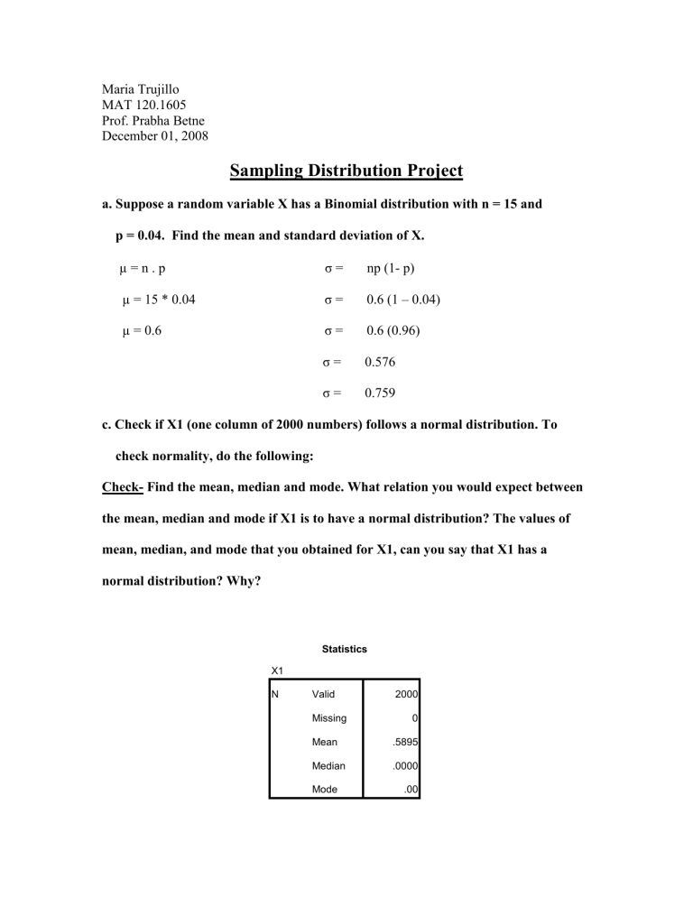
Check- Find the mean, median and mode. What relation you would expect between the mean, median and mode if X1 is to have a normal distribution? The values of mean, median, and mode that you obtained for X1, can you say that X1 has a normal distribution? Why?
X1
Statistics
N Valid 2000
Missing
Mean
Median
Mode
0
.5895
.0000
.00

Being the values of Mean= .5895, Median=.0000 and Mode= .00 do not have a normal distribution because they are not the same or very close.
Check-ii Obtain a histogram of X1 values and discuss the shape of the histogram.
Does the shape of histogram suggest that X1 has a normal distribution?
1200
1000
800
600
400
200
Std. Dev = .76
Mean = .6
N = 2000.00
0
0.0
1.0
2.0
3.0
4.0
5.0
X1
No, it does not suggest that X1 has a normal distribution because the graph is left skewed.
This means that most of the data falls to the left side.
Check-iii Obtain a Normal QQ plot (Lesson 10) of the X1 values. Does the plot indicate that X1 has a normal distribution? Explain why.

3.5
3.0
2.5
2.0
1.5
1.0
.5
0.0
-1 0
Observed Value
1 2 3 4 5 6
2.0
1.5
1.0
.5
0.0
-.5
-1 0
Observed Value
1 2 3 4 5 6

From the above plot, the scores do not appear to be from a normal distributed population because most of the data is outling. d. Now assuming each row is a sample of size 30, find the mean of each row. e. Check if the means that you computed in part (d) follow a normal distribution.
Follow the same three checks as you did for part (c).
Statistics
MEAN
N Valid 2000
Missing
0
Mean .5943
Median
.6000
Mode .57
400
300
200
100
0
.19
.25
.31
.38
.44
.50
.56
.63
.69
.75
.81
.88
.94
1.00
1.06
Std. Dev = .14
Mean = .59
N = 2000.00
MEAN

1.2
1.0
.8
.6
.4
.2
0.0
0.0
.2
Observed Value
.4
.6
.8
1.0
1.2
.05
.04
.03
.02
.01
0.00
-.01
0.0
.2
Observed Value
.4
.6
.8
1.0
1.2

f. In view of the central limit theorem, what did you expect the distribution of the
means to be? What mean and standard deviation values did you expect for the
means. (Compute this by hand)
x N (µ , σ ) σ =

30
µ = n * p
µ = 15 * 0.04 σ = 0.759
µ = 0.6 30
σ = 0.1386 g. Find the mean and standard deviation values of the means column and compare
with the value of mean and standard deviation that you discussed in part f.
Statistics
MEAN
N Valid
2000
Missing 0
Mean .5943
Median
.6000
Mode .57
Std. Deviation
.13712
The expected value of the Mean using the Central Limit Theorem is µ= 0.6 and
σ= 0.1368. We can notice that my answers are really close to the ones of the Mean of
Means computed in SPSS.
Write your understanding about the Central Limit Theorem (CLT). How did this project help you understand the CLT? How can you use this result for solving problems in statistics? You may use any example from the book to explain.

The Central Limit Theorem (CLT) says that regardless of the shape of the population when we have a large sample (more than 30) the sampling distribution of the data always is going to be normal. The CLT is very useful in solving statistics problems because even though the distribution of the data can not be normal as we can see in the tables above, if I have a large sample I can assume that the data that I have has a normal distribution without the necessity of solving for it. Even though the first tables do not have a normal distribution result we can notice that after computing the Mean of the
Means we get a outcome very close to the one that I computed by hand assuming that we have a normal distribution. The CLT is very handy for solving statistics problems because all I need to make sure that my sample is larger than 30 or if the population
Mean is normal to assume that I would have normal distribution.