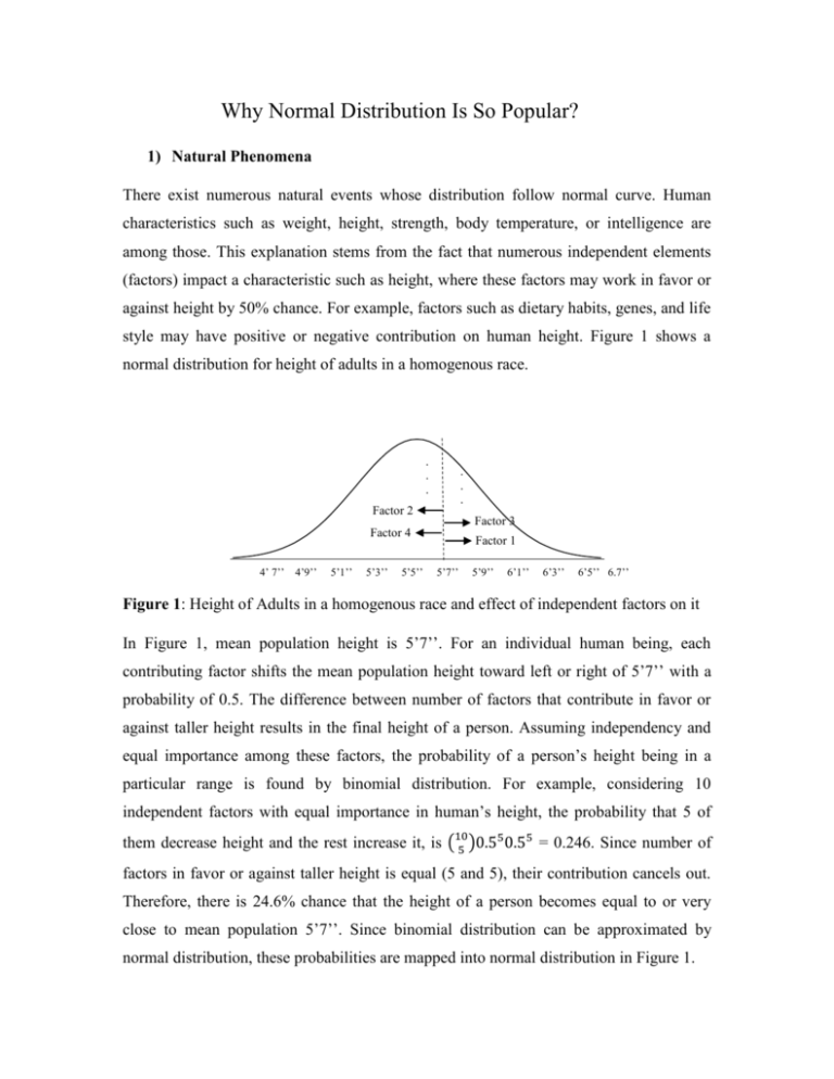
Why Normal Distribution Is So Popular?
1) Natural Phenomena
There exist numerous natural events whose distribution follow normal curve. Human
characteristics such as weight, height, strength, body temperature, or intelligence are
among those. This explanation stems from the fact that numerous independent elements
(factors) impact a characteristic such as height, where these factors may work in favor or
against height by 50% chance. For example, factors such as dietary habits, genes, and life
style may have positive or negative contribution on human height. Figure 1 shows a
normal distribution for height of adults in a homogenous race.
.
.
.
.
.
.
Factor 2
Factor 3
Factor 4
4’ 7’’ 4’9’’
5’1’’
5’3’’
5’5’’
Factor 1
5’7’’
5’9’’
6’1’’
6’3’’
6’5’’ 6.7’’
Figure 1: Height of Adults in a homogenous race and effect of independent factors on it
In Figure 1, mean population height is 5’7’’. For an individual human being, each
contributing factor shifts the mean population height toward left or right of 5’7’’ with a
probability of 0.5. The difference between number of factors that contribute in favor or
against taller height results in the final height of a person. Assuming independency and
equal importance among these factors, the probability of a person’s height being in a
particular range is found by binomial distribution. For example, considering 10
independent factors with equal importance in human’s height, the probability that 5 of
them decrease height and the rest increase it, is (10
)0.55 0.55 = 0.246. Since number of
5
factors in favor or against taller height is equal (5 and 5), their contribution cancels out.
Therefore, there is 24.6% chance that the height of a person becomes equal to or very
close to mean population 5’7’’. Since binomial distribution can be approximated by
normal distribution, these probabilities are mapped into normal distribution in Figure 1.
2) Manufacturing/Service Industry
Numerous features in manufacturing and service industries follow normal distribution.
For example, two important service indices in a shipping company is the mean and
standard deviation of delivery time. These two indices can be explained by a normal
curve with mean and standard deviation of delivery time. Mean and standard deviation of
service time in cleaning companies is another example of the phenomena with normal
distribution.
3) Central Limit Theorem (CLT)
CLT explains that there is a strong relation between sample size and the extent to which a
sampling distribution resembles normal curve. Batch size samples are large enough so
that their weight, volume, or dimension can be approximated by normal distribution even
though the population distribution itself is not normal. In order to use CLT, measurement
results needs to be reported as an aggregated value. For example in continuous
production lines such as beverage, steel, or oil industry, weight of product is measured
per batch (bar or barrel). There are practical justifications behind this measuring method
such as reducing direct costs and inspectors’ working hours. However, one important
advantage is that aggregated measures follow normal distribution, no matter what
distribution each individual observation has. Therefore, quality control team who inspects
these features in production lines take advantage of CLT to inspect these properties as an
aggregated value for the whole batch.
4) Independence of Distribution Parameters (µ, σ)
In contrast with binomial or exponential distributions, parameters of normal distribution
are independent from each other. As a result of this interesting property, if any error
occurs in measuring population mean, µ, it does not affect standard deviation measure, σ.
σ is also considered as the quality measure. This independency does not exist in
regression parameters b0 and b1. This is because b0 is estimated as function of b1, b0 =


y  b1 x