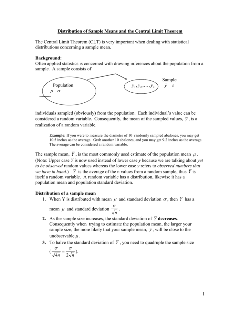
Distribution of Sample Means and the Central Limit Theorem
The Central Limit Theorem (CLT) is very important when dealing with statistical
distributions concerning a sample mean.
Background:
Often applied statistics is concerned with drawing inferences about the population from a
sample. A sample consists of
y1 , y 2 ,  , y n
Population
 
Sample
y s
individuals sampled (obviously) from the population. Each individual’s value can be
considered a random variable. Consequently, the mean of the sampled values, y , is a
realization of a random variable.
Example: If you were to measure the diameter of 10 randomly sampled abalones, you may get
10.5 inches as the average. Grab another 10 abalones, and you may get 9.2 inches as the average.
The average can be considered a random variable.
The sample mean, Y , is the most commonly used estimate of the population mean  .
(Note: Upper case Y is now used instead of lower case y because we are talking about yet
to be observed random values whereas the lower case y refers to observed numbers that
we have in hand.) Y is the average of the n values from a random sample, thus Y is
itself a random variable. A random variable has a distribution, likewise it has a
population mean and population standard deviation.
Distribution of a sample mean
1. When Y is distributed with mean  and standard deviation  , then Y has a
mean  and standard deviation

.
n
2. As the sample size increases, the standard deviation of Y decreases.
Consequently when trying to estimate the population mean, the larger your
sample size, the more likely that your sample mean, y , will be close to the
unobservable  .
3. To halve the standard deviation of Y , you need to quadruple the sample size
(

4n


2 n
).
1
4. In practice, you do not know  , so you calculate s.
error of the sample mean. It an estimate of

s
is called the standard
n
.
n
Knowing the distribution of Y allows you to answer many practical questions using
statistics. Each population, whether it be red abalone shell diameters, weight of people,
river water flow, or tree heights certainly has its own unique probability distribution. (To
really take advantage of statistics, you need to think of most objects in nature as being an
observation of a random variable.) So how can you possibly know the distribution of the
sample mean Y if you do not know the true distribution of the population? In many
cases, the distribution of Y is known because of the Central Limit Theorem.
The Central Limit Theorem (CLT) deals with the distribution of Y . The is very
important when dealing with statistical distributions concerning a sample mean.
Central Limit Theorem
Suppose Y has most any distribution with mean  and standard deviation  . Then, as n
gets large, the distribution of Y will become “approximately normal” with mean  and
standard deviation

n
. The larger n, the closer the distribution of Y will be to being
normal.
Note1: If Y is a normal distribution, then the distribution of Y is normal regardless of n.
Note2: There are very rare instances where the CLT fails, but the distribution must have
infinite values with non-zero probability – don’t worry about encountering this.
When “n gets large” is large enough depends upon how different the Y’s
distribution is from normal. Typically n=30 is used as a rough guideline.
Remember, it is the distribution of the sample means that become approximate
normal – the distribution of the individuals in the population does not change.
Why is the CLT important? Statistical tests, such as a t-test or Analysis of Variance
(ANOVA) assume that the data were sampled from a normal population, thus giving
an Y that is normally distributed. Y , however, can be assumed to be normally distributed
if n is large because of the CLT. Consequently, for “large” sample sizes the issue of
whether or not the population is normally distributed is not a concern. Thus the CLT
permits use of t-tests and ANOVA when the population is non-normal. Similarly this is
true for confidence intervals for the population mean  .
Example: Suppose Gambel Quail lay an average of 14 eggs in a clutch with a standard deviation
of 2. Obviously the number of eggs cannot be normally distributed because the number of eggs is
a discrete, not continuous, random variable. Furthermore, it is safe to assume that the number of
eggs is probably skewed either to the left or right.
Suppose many students were to go out and count the eggs in 50 different Gambel Quail clutches
and calculate the average number of eggs in a clutch. What would be the distribution that these
2
averages follow? Answer: Because n=50 is “large”, the distribution of the mean number of eggs
would be approximately normal with
 x  14 and  x 
2
 0.28 .
50
Example:
Here we have the density curve
for a chi-square distribution
with 6 degrees of freedom.
Obviously not normal, but not
does have a bit of bell-shaped
curve to it. Consequently, the
distribution of it’s sample
means approaches a normal
distribution with relatively
small sample sizes.
the sample mean.
3
Example: The CLT will even work with a discrete distribution, such as rolling a die.
The probabilities for 1 through 6 are equal. Roll the die n times and average those rolls –
if n is large, we can consider the average to be a random variable from a normal
distribution.
4