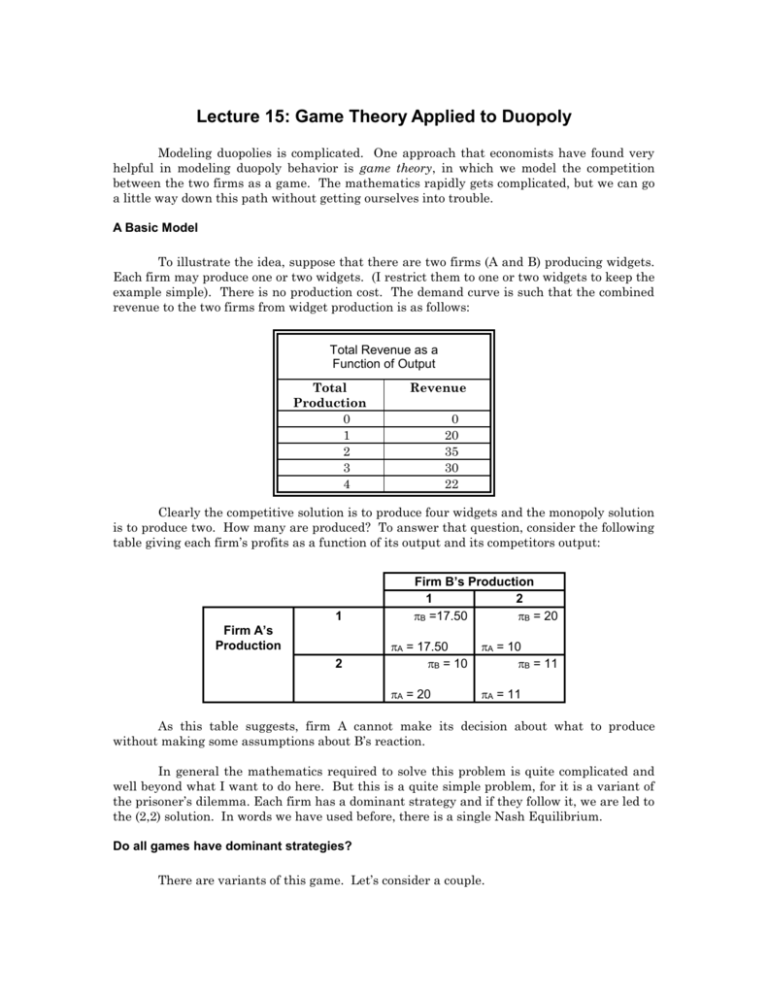
Lecture 15: Game Theory Applied to Duopoly
Modeling duopolies is complicated. One approach that economists have found very
helpful in modeling duopoly behavior is game theory, in which we model the competition
between the two firms as a game. The mathematics rapidly gets complicated, but we can go
a little way down this path without getting ourselves into trouble.
A Basic Model
To illustrate the idea, suppose that there are two firms (A and B) producing widgets.
Each firm may produce one or two widgets. (I restrict them to one or two widgets to keep the
example simple). There is no production cost. The demand curve is such that the combined
revenue to the two firms from widget production is as follows:
Total Revenue as a
Function of Output
Total
Production
0
1
2
3
4
Revenue
0
20
35
30
22
Clearly the competitive solution is to produce four widgets and the monopoly solution
is to produce two. How many are produced? To answer that question, consider the following
table giving each firm’s profits as a function of its output and its competitors output:
1
Firm A’s
Production
2
Firm B’s Production
1
2
B =17.50
B = 20
A = 17.50
B = 10
A = 10
B = 11
A = 20
A = 11
As this table suggests, firm A cannot make its decision about what to produce
without making some assumptions about B’s reaction.
In general the mathematics required to solve this problem is quite complicated and
well beyond what I want to do here. But this is a quite simple problem, for it is a variant of
the prisoner’s dilemma. Each firm has a dominant strategy and if they follow it, we are led to
the (2,2) solution. In words we have used before, there is a single Nash Equilibrium.
Do all games have dominant strategies?
There are variants of this game. Let’s consider a couple.
One firm has a dominant strategy; the other does not
Here is a simple example. Firm 1 is an automobile company with great engineering
skills. Firm 2 has good designers and does great styling. Yet both firms have the capability
of doing either one. They cannot do both. The payoff matrix looks like the following:
Firm 1’s
choices
Technical
Model
Change
Styling
Model
Change
Firm 2’s choices
Technical
Styling
model
model
change
change
2 =20
2 = 15
1 = 40
2 = 16
1 = 60
2 = 18
1 = 8
1 = 12
Firm 1 has a dominant strategy: the technical model change. Firm 2, however, does
not have a dominant strategy. Still, Firm 2 choice is obvious. It should assume that Firm 1
would adopt its rational choice, the technical model change; it would therefore be advised to
go itself with the technical model change. The lesson: assume your opponent will act
rationally.
Here is a second example. Firms have a choice of when to enter a new brand, early or
late. Firm 1 has a well-established well-recognized brand in another market, and wants to
take advantage by introducing a product in this new market by using the existing name, the
so-called brand extension strategy. (E.g., Coke introducing Diet Coke). But because its
existing brand is profitable, it runs the risk of damaging its brand if the new product fails.
The second firm does not have the fortune of having an established brand, and
therefore runs no risk of ruining its existing brand. It is generally better off introducing
early. The payoff matrix is as follows:
Firm 1’s
choices of
When to
extend the
brand
Early entry
Firm 2’s choices of when to
enter the new brand
Early entry
Late entry
2 =60
2 = 20
Late entry
1 = 40
2 = 80
1 = 45
2 = 55
1 = 95
1 = 35
The second firm has a dominant strategy: early entry. The first firm does not. But
given the second firm’s dominant strategy, the established firm is justified in waiting.
Multiple Nash Equilibria
It is also possible to have multiple equilibria. Let’s change the payoff matrix for the
styling change to read as follows:
Firm 1’s
choices
Technical
Model
Change
Styling
Model
Change
Firm 2’s choices
Technical
Styling
model
model
change
change
2 =20
2 = 55
1 = 20
2 = 60
1 = 60
2 = 25
1 = 55
1 = 25
In this case, neither firm has a dominant strategy. But there are two Nash
equilibria, indicated by boldfacing the choices. The firm that first announces a technical
model change wins the race, and thus both firms want to be the first to announce.
Repeated Games
Twelve years ago, I would have ended discussion of game theory issues at this point.
But there is new research, and leads us to strategies for repeated games. Here it now
becomes optimal to adopt what is either called a tit for tat strategy or punishment strategy.
Suppose two firms are producing a product. The total demand is
q = 100-2p
The marginal cost is $5, so that the monopoly solution is to sell the product at $27.50, and
split the market for 45 units between them. If they do so, they earn combined profits of
($22.50)(45) = $1012.50. One half of that would be $506.25. But each firm knows that if it
cuts its price by one penny to $24.49, it can capture the whole market and essentially double
their profits. Thus Firm 1, for instance, has a strong incentive to cheat. Indeed, it may fear
that if it doesn't cheat first, Firm 2 will simply beat it to the punch.
There is a counter-strategy for Firm 2. It can announce or signal that, if Firm 1 does
that, it will respond by cutting its price to $5 forever thereafter. Thus Firm 1 can choose
between two strategies:

Charge the monopoly price period after period and earn $512.50 per period.

Cheat for one period.
nothing thereafter.
Earn twice that amount for one period, but earn
Given this option, Firm 1 will not want to cut price.
Does this strategy work? This is essentially the idea behind Mutual Assured
Destruction, the policy used by the United States and the Soviet Union during the Cold War.
We told the Soviets that, if they dropped nuclear weapons on us, or if they invaded Western
Europe, we would unleash our nuclear arsenal on them. They replied in kind.
A variant of this is the simple tit-for-tat strategy. In this case, Firm 2 responds with
the threat of cutting its price to $5, but only for one period. Then Firm 1 is indifferent
between cheating on the monopoly price and not cheating. The general strategy is the
following:
What Firm 1 Did Last Period?
Firm 2’s Strategy this Period
Followed the Cooperative Strategy
Follow the Cooperative Strategy
Followed the Non-cooperative Strategy
Follow the Non-cooperative Strategy
We call this the tit-for-tat strategy. Mathematical economists have not been able to
prove that this is the best strategy, but no one has yet found a case where it doesn’t work.
Thus we believe, though we cannot show this is the optimal way to deal with non-cooperative
behavior.
Sequential Games
The previous example suggests what economists call sequential games. Firm 1
undertakes some action, such as cutting price. Firm 2 then follows in the next time period
with another decision. Many of the problems that we have talked about are really sequential
games. We will now analyze them explicitly with what economists call a game tree.
Figure 15-1 illustrates a particular problem. An entrant is considering entering a
new business. After it enters, or doesn’t, the incumbent can either expand or maintain his
capacity. In short, the decisions are sequential. The incumbent threatens that it will expand
capacity should the new firm enter the business. If it does so, the new firm will lose money.
How seriously should the new firm take the threat from the existing firm? Is this a
credible threat or merely a bluff? Economists would propose a simple test:

Suppose the new firm enters the business. Is it then in the interest of the
existing firm to expand? If so, the threat to expand is credible. If not, it is simply
a bluff.
That is, the strategy is to assume that the existing firm will follow the strategy that
is in his or her best interest once the new firm has made its decision.
In this case, the threat by the existing firm is just that. It is not a credible threat. If
the new firm enters the business, the existing firm is better off not expanding capacity. Thus
the entrant will not be deterred. The reason is quite simple. No matter what the Incumbent
threatens or promises it will ultimately act in its self-interest. And, since it doesn't act until
after the Entrant has made her decision, the Incumbent, given these payoffs, will find it
optimal to expand if and only if the Entrant does not enter the business.
Thus the Entrant must analyze the Incumbent's incentives and assume rational
behavior on the part of the Incumbent. When she does so, she will not believe the
Incumbent's threat.
A Sequential Game
A potential entrant is considering entering the industry. The
incumbent threatens to expand capacity whether the new entrant
enters or not.
But the potential entrant does not view the
incumbent's threat to expand capacity in the event of entry as
credible. The payoffs are (Entrant, Incumbent)
How can the incumbent firm make its threat credible? There are a number of ways it
can do so. It could, for example, sign a binding contact on a new building. Suppose, for
example, it spends $15 on a new building. If it actually expands, the money is not lost. If it
doesn’t the money is lost forever. Now the payoff matrix looks like that illustrated in Figure
15-2. As you can see, the threat is now credible. This explains why firms must sometimes
make some actions and why it is important that they be public.
An Altered Game
By spending $15 towards expansion that it cannot recover, the
incumbent has converted its threat to expand the business into a
credible threat. The new payoffs are shown, with the old payoffs
crossed out. Now, if it does not expand, it loses the $15 investment
Finally, let me consider another example that illustrates how our laws influence
credible commitments. I hire you to do work around my house. You value your time at $40,
and I value having the work done at $60. You and I reach agreement for me to pay $50 after
the work is done. You have two choices. You can do the work or you cannot. I also have two
choices: I can pay you or not. If there is no law requiring me to pay you, then the sequential
game looks like that illustrated in Figure 15-3.
The Contracting Problem
A homeowner hires someone to work at his house, agreeing to pay
$50. The homeowner values the work at $60 and the worker values
the lost leisure at $40. Hence the makings of a bargain. But the
homeowner has the option of paying or not paying. Absent any legal
restrictions, the homeowner will not pay. The promise to pay is not
credible, and the homeowner will thus not get the work done.
Given these incentives, my dominant strategy is not to pay you, and you, knowing
this, will not be willing to do the work. (You may object that there is a more complicated
game involving reputation, etc., but that is another issue).
Finally, suppose that, if you do the work and I do not pay you, then you can sue me
for the $50 as well as $25 in damages. (Why $25? Why not?) The game now changes to be
like that illustrated in Figure 15-4. Now, you will do the work.
The Contracting Problem With
Legal Recourse
A homeowner hires someone to work at his house, agreeing to pay
$50. The homeowner values the work at $60 and the worker values
the lost leisure at $40. Hence the makings of a bargain. But the
homeowner has the option of paying or not paying. Absent any legal
restrictions, the homeowner will not pay. The promise to pay is not
credible, and the homeowner will thus not get the work done.
Now suppose that, if the worker is not paid, he can sue for the $50
plus $25 in punitive damages. Now the payoff matrix changes
dramatically, and the deal will be struck.
Uncertainty about the numbers
You may also ask how this would all change if the numbers were uncertain. If the
uncertainty is small, the numbers will not change much and thus the strategy will still
remain the same. True uncertainty is more complicated.
Minimax Strategies
There are more complicated models that we can analyze with game theory, and I
want to give one to illustrate the basic concept. To do so, we need to define a zero-sum game,
in which one firm’s profits are another firm’s losses. Flipping coins or other betting games
are straightforward examples of zero-sum games. While they don’t often arise in Economics
(most people prefer to pay positive sum games such as buying a product - which generates
both consumer and producer surplus), the mathematicians assure us that

Zero sum games are easier to analyze; and

Positive sum games can easily be converted to zero sum games and vice versa.
Consider, for example, the following pay-off matrix for a zero sum game involving A
and B. Since this is a zero-sum game, we only display A’s gains, for B’s losses are exactly the
opposite of A’s gains.
If B Follows Strategy
If A Follows Strategy
B1
B2
A1
1
2
A2
3
1
Clearly there is not a dominant strategy here. If A always follows strategy A 1, then B
will always follow B1. On the other hand, if A always follows strategy A 2, then B will always
follow B2. That would suggest that A can only win $1.
Choosing B’s optimal Strategy
But suppose that A follows a mixed strategy. That is, part of the time, A follows
strategy A1 and the other times, strategy A2. Clearly A will do better with this mixed
strategy. It will always win $1 and sometimes $2 or $3, depending on what B does.
Now see what happens to B’s strategies. When it follows B 1, it will lose $1 part of the
time and $3 part of the time. When it follows B 2, it loses $2 part of the time and $1 part of
the time. The correct solution is to follow B1 p1 percent of the time and B2 (1-p1) percent of
the time. In that case, A’s winnings are
From Strategy A1
p1 (1) + (1-p1)(2)
From Strategy A2
p1 (3) + (1-p1) (1)
The payoffs to A depend on what B does. Here are some typical payoffs:
Payoff from Strategy
p1 = 1.0
P1 = 2/3
p1 = 1/3
p1 = 0
A1
1
4/3
5/3
2
A2
3
7/3
5/3
1
As you can see, the maximum winnings that A can get from following either strategy
A1 or strategy A2 is minimized when p1 = 1/3. That turns out to be the best B can do. Note
that it does not know what A will do, but it has followed a strategy that minimizes its
maximum games, a so-called minimax strategy.
The minimax strategy turns out to be the best that can be done. There is an obvious
analogy to playing poker. If you always fold a poor hand and raise a good hand, you will not
make much money. You must, on occasion, bet on a poor hand and fold on a good hand. If
not, your opponent can “read” your bets and adjust his accordingly.
Any attempt to carry this further will lead us into advanced mathematics. But this
quick introduction will illustrate what can be one to set up strategy problems in a game
theoretic framework.
There is a simple graphical way to solve this problem. Figure 13-5 plots the payoff
functions for each of A’s strategies. A little paranoia on B’s part is called for. As you can see,
B minimizes A’s maximum gains by playing strategy B1 1/3 of the time.
Mini-max Payoffs in Game Theory
B is going to follow strategy B1 p1 percent of the time and B2 (1-p1)
percent of the time. How should p1 be chosen?
To answer, we must consider A's strategy. This graph plots A's
winnings from strategies A1 and A2 as a function of p2, the percent of
the time A follows strategy A1. At p1=0, for instance, A's payoff from
strategy A1 is 2. This would be the optimal strategy for A if B
followed B2 all of the time. If p1=1, so that B followed B1 all of the
time, A's optimal strategy would change. B can ensure that A's
maximum winnings are minimized by setting p 1 = 1/3. This is called
the minimax strategy.
In commonsense terms, the minimax strategy is to assume you have
an intelligent opponent and set your plans assuming optimal
behavior on his part.