Testing equality of variance:
In statistics, when a usual regression or one-way ANOVA is performed, it is assumed
that the group variances are statistically equal. If this assumption is not valid, then the
resulting F-test is invalid.
Bartlett's test (Snedecor and Cochran, 1983) is used to test if k samples have equal
variances. Equal variances across samples is called homoscedasticity or homogeneity of
variances. Some statistical tests, for example the analysis of variance, assume that
variances are equal across groups or samples. The Bartlett test can be used to verify that
assumption.
Bartlett's test is sensitive to departures from normality. That is, if your samples come
from non-normal distributions, then Bartlett's test may simply be testing for nonnormality. The Levene test and Brown-Forsythe test are alternatives to the Bartlett test
that are less sensitive to departures from normality.
Bartlett's test is used to test the null hypothesis, H0 that all k population variances are
equal against the alternative that at least two are different.
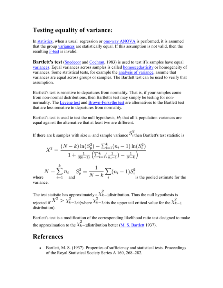
If there are k samples with size ni and sample variance
then Bartlett's test statistic is
where
variance.
is the pooled estimate for the
and
The test statistic has approximately a
rejected if
distribution).
(where
distribution. Thus the null hypothesis is
is the upper tail critical value for the
Bartlett's test is a modification of the corresponding likelihood ratio test designed to make
the approximation to the
distribution better (M. S. Bartlett 1937).
References

Bartlett, M. S. (1937). Properties of sufficiency and statistical tests. Proceedings
of the Royal Statistical Society Series A 160, 268–282.

Snedecor, George W. and Cochran, William G. (1989), Statistical Methods,
Eighth Edition, Iowa State University Press.
The Brown-Forsythe test is a statistical test for the equality of group variances based
on performing an ANOVA on a transformation of the response variable.
Transformation
The transformed response variable is constructed to measure the spread in each group.
Let
where is the median of group j. In order to correct for the artificial zeros that come
about with odd numbers of observations in a group, any zij that equals zero is replaced by
the next smallest zij in group j. The Brown-Forsythe test statistic is the model F statistic
from a one way ANOVA on zij:
where p is the number of groups, nj is the number of observations in group j, and N is the
total number of observations.
If the variances are indeed heterogeneous, techniques that allow for this (such as the
Welch one-way ANOVA) may be used instead of the usual ANOVA.
****************************************
LEVENE TEST
Name:
LEVENE TEST
Type:
Analysis Command
Purpose:
Perform a k-sample Levene test for the homogeneity of variances across
samples.
Description:
The F test used in analysis of variance problem with k factors can be
sensitive to unequal standard deviations in the k factors. Levene's test is a
test of the hypothesis that all factor standard deviations (or equivalently
variances) are equal against the alternative that the standard deviations
are not all equal.
The assumption of homogeneous variances arises in other contexts in
addition to analysis of variance. Levene's test can be applied in these
cases as well.
The Levene test is an alternative to the Bartlett test. Although it is more
commonly used, the Bartlett test is known to be sensitive to departures
from normality. The Levene test is less sensitive to non-normality than the
Bartlett test.
The Levene test is defined as:
H0:
Ha:
Test
Statistic:
for at least one pair (i,j).
Given a variable Y with sample of size N divided into k sub-groups,
where Ni is the sample size of the ith sub-group, the Levene test
statistic is defined as:
where Zij can have one of the following three definitions:
1.
where
2.
is the mean of the ith subgroup.
where
is the median of the ith subgroup.
where
is the 10% trimmed mean of the ith subgroup.
3.
are the group means of the Zij and
is the overall mean of the Zij.
The three choices for defining Zij determine the robustness and
power of Levene's test. By robustness, we mean the ability of the test
to not falsely detect non-homogeneous groups when the underlying
data is not normally distributed and the groups are in fact
homogeneous. By power, we mean the ability of the test to detect
non-homogeneous groups when the groups are in fact nonhomogenous.
The definition based on the median is recommended as the choice
that provides good robustness against many types of non-normal
data but retains good power.
Significance (typically 0.05).
Level:
Critical
The Levene test rejects the hypothesis that the variances are
Region:
homogeneous if
where
is the upper critical value of the F distribution
with k - 1 and N - 1 degrees of freedom at a significance level of .
Syntax 1:
LEVENE TEST <y> <tag> <SUBSET/EXCEPT/FOR qualification>
where <y> is a response variable;
<tag> is a factor identifier variable;
and where the <SUBSET/EXCEPT/FOR qualification> is optional.
This syntax computes the median based Levene test.
Syntax 2:
MEDIAN LEVENE TEST <y> <tag> <SUBSET/EXCEPT/FOR
qualification>
where <y> is a response variable;
<tag> is a factor identifier variable;
and where the <SUBSET/EXCEPT/FOR qualification> is optional.
This syntax computes the median based Levene test.
Syntax 3:
MEAN LEVENE TEST <y> <tag> <SUBSET/EXCEPT/FOR qualification>
where <y> is a response variable;
<tag> is a factor identifier variable;
and where the <SUBSET/EXCEPT/FOR qualification> is optional.
This syntax computes the mean based Levene test.
Syntax 4:
TRIMMED MEAN LEVENE TEST <y> <tag> <SUBSET/EXCEPT/FOR
qualification>
where <y> is a response variable;
<tag> is a factor identifier variable;
and where the <SUBSET/EXCEPT/FOR qualification> is optional.
This syntax computes the trimmed mean based Levene test. It trims the
lowest 10% and the highest 10% of the data.
Examples:
LEVENE TEST Y1 GROUP
LEVENE TEST Y1 GROUP SUBSET GROUP > 2
MEDIAN LEVENE TEST Y1 GROUP
MEAN LEVENE TEST Y1 GROUP
TRIMMED MEAN LEVENE TEST Y1 GROUP
Note:
The various values printed by the LEVENE TEST command are saved as
parameters that can be used later by the analyst. Enter the command
STATUS PARAMETERS after the LEVENE TEST command to see a list
of the saved parameters.
Note:
The HOMOGENEITY PLOT is a graphical technique for testing for
unequal variances.
Default:
The default is to to compute the Levene test based on group medians.
Synonyms:
None
Related Commands:
BARTLETT TEST
= Compute Bartlett's test.
HOMOGENEITY
= Plot group standard deviations against group means.
PLOT
CONFIDENCE
= Compute the confidence limits for the mean of a
LIMITS
sample.
F TEST
= Performs a two-sample F test.
T TEST
= Performs a two-sample t test.
= Performs a one sample chi-square test that the standard
CHI-SQUARE TEST
deviation is equal to a given value.
STANDARD
= Computes the standard deviation of a variable.
DEVIATION
Reference:
Levene, H. (1960). "Contributions to Probability and Statistics: Essays in
Honor of Harold Hotelling", I. Olkin, et. al., eds. Stanford University Press,
Stanford, CA, pp. 278-292.
Applications:
Analysis of Variance, Regression
Implementation Date:
1998/5
Program:
SKIP 25
READ VANGEL32.DAT Y X BATCH
.
LEVENE TEST Y X
STATUS PARAMETERS
Dataplot generated the following output:
**************************
**
LEVENE TEST Y X **
**************************
LEVENE F-TEST FOR SHIFT IN VARIATION
(ASSUMPTION: NORMALITY)
1. STATISTICS
NUMBER OF OBSERVATIONS =
45
NUMBER OF GROUPS
=
3
LEVENE F TEST STATISTIC = 10.88619
FOR LEVENE TEST STATISTIC
0
% POINT =
0.
50
% POINT = 0.7047137
75
% POINT = 1.433075
90
% POINT = 2.433564
95
% POINT = 3.219942
99
% POINT = 5.149141
99.9
% POINT = 8.179383
99.98448
% Point:
10.88619
3. CONCLUSION (AT THE 5% LEVEL):
THERE IS A SHIFT IN VARIATION.
THUS: NOT HOMOGENOUS WITH RESPECT TO VARIATION.
PARAMETER INFINITY HAS THE VALUE:
0.3402823E+39
PARAMETER PI
HAS THE VALUE: 0.3141593E+01
PARAMETER STATVAL HAS THE VALUE: 0.1088619E+02
PARAMETER STATCDF HAS THE VALUE: 0.9998448E+00
PARAMETER CUTOFF0 HAS THE VALUE: 0.0000000E+00
PARAMETER CUTOFF50 HAS THE VALUE: 0.7047137E+00
PARAMETER CUTOFF75 HAS THE VALUE: 0.1433075E+01
PARAMETER CUTOFF90 HAS THE VALUE: 0.2433564E+01
PARAMETER CUTOFF95 HAS THE VALUE: 0.3219942E+01
PARAMETER CUTOFF99 HAS THE VALUE: 0.0000000E+00
PARAMETER CUTOF999 HAS THE VALUE: 0.0000000E+00
*********************************************
Comparison of Brown-Forsythe test with Levene's test
Levene's test uses the mean instead of the median. Although the optimal choice depends
on the underlying distribution, the definition based on the median is recommended as the
choice that provides good robustness against many types of non-normal data while
retaining good statistical power. If one has knowledge of the underlying distribution of
the data, this may indicate using one of the other choices. Brown and Forsythe performed
Monte Carlo studies that indicated that using the trimmed mean performed best when the
underlying data followed a Cauchy distribution (a heavy-tailed distribution) and the
median performed best when the underlying data followed a Chi-square distribution with
four degrees of freedom (a heavily skewed distribution). Using the mean provided the
best power for symmetric, moderate-tailed, distributions.
References

Brown, Morton B. and Forsythe, Alan B. (1974), Robust Tests for Equality of
Variances, Journal of the American Statistical Association, 69, 364-367.
***************************************************
We can also use the Breusch-Pagan
error variance.
Test to formally test the constancy of
The Breusch-Pagan test is a large-sample test for constancy of error variance. It
assumes that error terms are independent and normally distributed and that the
variance of the error term i, denoted by  i2 , is related to the levels of q predictor
variables in the following way:
log e ( i2 )   0  1X i1    q X iq
Note that above equation implies that  i2 either increases or decreases with the level
of the q predictor variables, depending on the sign of s. Constancy of error variance
corresponds to  1   2    q  0 . Therefore a test of H0:  1   2    q  0 can be
carried out by
(1) fitting the following regression model :
log e (e i2 )   0  1X i1    q X iq   i
where i is the error term for this regression model. The regression sum of squares
can then be obtained and denoted by SSR*.
(2) obtain SSE, the error sum of squares from the following regression model:
Yi   0  1 X i1   q X iq   i
SSR * / q
, which follows approximately the chi(SSE / n) 2
square distribution with q degree of freedom when  1   2    q  0 holds and n is
(3) calculate the test statistic  2BP 
reasonably large
(4)
 2BP   2  1  , q   H 0 :1   2  q  0 
 2   2  1  , q   reject H

 BP

0
or

pvalue   H 0 : 1   2   q  0
2
BP    reject H 0

SAS CODE: : In a small-scale experimental study of the relation between degree
of brand liking (Y) and moisture content (X1) and sweetness (X2) of the product,
the data were obtained from the experiment based on a completely randomized
design, see CH06PR05.txt from your textbook..
data Brandpreference;
infile 'Z:\ch06pr05.txt';
input y x1 x2;
proc reg data=Brandpreference;
model y=x1 x2/r p;
output out=results r=residual p=yhat;
run;
data results;
set results;
e2 = residual*residual;
proc reg data=results;
model e2 = x1 x2;
run;
quit;
SAS OUTPUT
Analysis of Variance
Source
DF
Sum of
Squares
Mean
Square
Model
Error
Corrected Total
2
13
15
1872.70000
94.30000
1967.00000
936.35000
7.25385
Root MSE
Dependent Mean
Coeff Var
2.69330
81.75000
3.29455
R-Square
Adj R-Sq
F Value
Pr > F
129.08
<.0001
0.9521
0.9447
Parameter Estimates
Variable
DF
Parameter
Estimate
Standard
Error
t Value
Pr > |t|
Intercept
x1
x2
1
1
1
37.65000
4.42500
4.37500
2.99610
0.30112
0.67332
12.57
14.70
6.50
<.0001
<.0001
<.0001
The REG Procedure
Model: MODEL1
Dependent Variable: e2
Number of Observations Read
Number of Observations Used
16
16
Analysis of Variance
Source
DF
Sum of
Squares
Mean
Square
Model
Error
Corrected Total
2
13
15
72.40700
494.34723
566.75423
36.20350
38.02671
Root MSE
Dependent Mean
Coeff Var
6.16658
5.89375
104.62914
R-Square
Adj R-Sq
F Value
Pr > F
0.95
0.4113
0.1278
-0.0064
Parameter Estimates
Variable
DF
Parameter
Estimate
Standard
Error
t Value
Pr > |t|
Intercept
x1
x2
1
1
1
1.15875
0.91750
-0.56250
6.85989
0.68944
1.54165
0.17
1.33
-0.36
0.8685
0.2061
0.7211
For this example, please conduct the Breusch-Pagan test for constancy of the
error variance, assuming log e ( i2 )   0   1 X i1   2 X i 2 ; use =0.01. State the
alternatives, decision rule and conclusion.
Lack of Fit Test
To ascertain whether a linear regression function is a good fit for the data, we can
carry out a formal test called lack of fit F-test. The lack of fit test assumes that the
observations Y for given predictor variables X1, X2, …, Xp-1 are (1) independent and (2)
normally distributed, and that (3) the distribution of Y have the same variance 2. The
lack of fit test requires repeat observations at one or more Xs levels. Lack of fit F-test is
a general linear test approach which compares the full model and reduced model:
Full model: Yij   j   ij
The full model states that each response Y is made up of two components: the mean
response when X1=X1j, X2=X2j,… , Xp-1=Xp-1j and a random error term.
Reduced Model: Yij   0  1X ij1   q X ijp1   ij
Note that here i refers to ith replicate observations, j refers to jth level of predictor
variable X1, X2, … Xp-1.
The difference between the full model and the reduced model is that in the full model
there are no restrictions on the mean I, whereas in the reduced model the mean
responses are linearly related to the Xs. A test statistic was then developed to compare
the error sum of squares from the full model and the reduced model as follows:
SSE (R )  SSE (F)
df R  df F
F* 
SSE (F) 
here
 (Y
ij
j
SSE (R ) 
SSE (F)
df F
 Yj ) 2 , df F  n  c
i
 (Y
ij
j
 (b 0  b1 X 1ij   b p 1 X p 1ij ) 2 , df R  n  p
i
F*  F1  ; c  p, n  c   conclude H 0 : E(Y)   0  1 X1   p-1 X p-1 
 *

F  F1  ; c  p, n  c   reject H 0

or
Pvalue    conclude H 0 : E(Y)   0  1 X 1   p-1 X p-1 


Pvalue    reject H 0

SAS CODE:
data Brandpreference;
infile 'c:\stat231B06\ch06pr05.txt';
input y x1 x2;
if x1=4 and x2=2 then j=1; /* create a new variable J*/
if x1=4 and x2=4 then j=2;
if x1=6 and x2=2 then j=3;
if x1=6 and x2=4 then j=4;
if x1=8 and x2=2 then j=5;
if x1=8 and x2=4 then j=6;
if x1=10 and x2=2 then j=7;
if x1=10 and x2=4 then j=8;
run;
proc glm data=Brandpreference;
class j;
model y= x1 x2 j;
run;
SAS OUTPUT:
The GLM Procedure
Class Level Information
Class
Levels
j
Values
8
1 2 3 4 5 6 7 8
Number of Observations Read
Number of Observations Used
16
16
The GLM Procedure
Dependent Variable: y
Source
DF
Sum of
Squares
Mean Square
F Value
Pr > F
Model
7
1910.000000
272.857143
38.30
<.0001
Error
8
57.000000
7.125000
15
1967.000000
Corrected Total
Source
x1
x2
j
R-Square
Coeff Var
Root MSE
y Mean
0.971022
3.265162
2.669270
81.75000
DF
Type I SS
Mean Square
F Value
Pr > F
1
1
5
1566.450000
306.250000
37.300000
1566.450000
306.250000
7.460000
219.85
42.98
1.05
<.0001
0.0002
0.4530
Source
DF
Type III SS
Mean Square
F Value
Pr > F
0
0
5
0.00000000
0.00000000
37.30000000
.
.
7.46000000
.
.
1.05
.
.
0.4530
x1
x2
j
To compute the Lack of fit F* in SAS, we switch to the proc glm procedure. We begin
by fitting the full model to the data. This requires creating a new variable, J. Using the
class j statement in proc glm , we specify that J is a classification variable. Thus, J
identifies 8 discrete classifications based on the values of Xs. The SAS output shows that
SSE(F)=57, SSE(R)-SSE(F)=37.3.
For this example, conduct a formal test for lack of fit of the first-order
regression function; use =0.01. State the alternatives, decision rule and
conclusion.
Joint Inference of several regression coefficients.
The Bonferroni joint confidence intervals can be used to estimate several regression
coefficients simultaneously. If g parameters are to be estimated jointly (where gp)), the
confidence limits with family confidence coefficient 1- are
b k  Bsb k 
B  t 1   2g ; n  p 
From
proc reg data=Brandference;
model y=x1 x2;
run;
We obtain the following estimates for regression coefficients and their corresponding
standard deviation.
Parameter Estimates
Parameter
Standard
Variable
DF
Estimate
Error
t Value
Pr > |t|
Intercept
x1
x2
1
1
1
37.65000
4.42500
4.37500
2.99610
0.30112
0.67332
12.57
14.70
6.50
<.0001
<.0001
<.0001
Then use the code below, we can estimate 1 and 2 jointly by the Bonferroni
procedure, using a 99 percent family confidence coefficient.
SAS CODE:
data intervals;
tvalue = tinv(.9975,13);
b1lo=4.425-(tvalue*0.30112);
b1hi=4.425+(tvalue*0.30112);
b2lo=4.375-(tvalue*0.67332);
b2hi=4.375+(tvalue*0.67332);
proc print;
var b1lo b1hi b2lo b2hi;
run;
/*lower
/*upper
/*lower
/*upper
bound
bound
bound
bound
for
for
for
for
b1*/
b1*/
b2*/
b2*/
SAS OUTPUT:
Obs
b1lo
b1hi
b2lo
b2hi
1
3.40948
5.44052
2.10425
6.64575
For this example, estimate  1 and  2 jointly by the Bonferroni procedure, using a
95 percent family confidence coefficient. Interpret your results.
Estimation of Mean Response and Prediction of New
Observation
A common objective in regression analysis is to estimate the mean for one or more
probability distribution of Y. Let X h1 , X h 2 ,..., X h ,p1 denote the level of Xs for which we
wish to estimate the mean response EYh  . X h1 , X h 2 ,..., X h ,p1 maybe a value which
occurred in the sample, or it may be some other value of the predictor variables within
the scope of the model. Ŷh is the point estimator of EYh  :

In terms of matrices:
 1 
 X 
h1 
Xh  
  
p1


X
 h ,p1 
EYh   Xh  (mean response)
Ŷh  Xh b
 
 Ŷ  X  bX   X XX  X
s Ŷ  X s bX  MSEX XX  X
E Ŷh  Xh  unbiased estimator of the mean response

2
h

1
2
h
h
h
h
1
2
h
h
h
h
 
Ŷh  t 1   2 ; n  p s Ŷh
Prediction of New Observation

Ŷh  t 1   2 ; n  p s Ŷh new 




s  Ŷh new   MSE 1  Xh XX  X h
1

h
SAS CODE for obtaining an interval estimate of EYh  Xh1=5 and Xh2=4, using a 99
percent confidence coefficient.
data Brandpreference;
infile 'Z:\ch06pr05.txt';
input y x1 x2;
tvalue = tinv(.995,13);/*find t-value for a t(13) with alpha=0.01*/
x0 = 1;
proc iml;
use Brandpreference;
read all var {'y'} into y;
read all var {'x1'} into a;
read all var {'x2'} into b;
read all var {'x0'} into con;
read all var {'tvalue'} into tvalue;
x=(con||a||b);
/*create X matrix*/
print x;
xtx=t(x)*x;
/*create X’X matrix*/
print xtx;
xty=t(x)*y;
/*create X’Y matrix*/
print xty;
b=inv(t(x)*x)*t(x)*y;/*create (X’X)^(-1)X’Y matrix*/
print b;
xtxinv=inv(t(x)*x); /*create (X’X)(-1) matrix*/
print xtxinv;
xh={1,5,4};
sxh=sqrt(7.25385*((t(xh))*(xtxinv)*xh)); /*7.25385 is MSE from*/
/*regression analysis*/
print sxh;
yhath = t(xh)*b;
print yhath;
yhathlo=yhath-(tvalue*sxh);
yhathhi=yhath+(tvalue*sxh);
low = yhathlo[1,1];
high=yhathhi[1,1];
print low high;
run;
quit;
SAS OUTPUT:
LOW
HIGH
73.881108 80.668892
For this example, obtain an interval estimate of EYh  Xh1=5 and Xh2=4, using a
95 percent confidence coefficient. Interpret your interval estimate
SAS CODE for obtain a prediction interval for a new observation Yh(new) when Xh1=5
and Xh2=4. Use a 99 percent confidence coefficient.
data Brandpreference;
infile 'Z:\ch06pr05.txt';
input y x1 x2;
b = tinv(.995,13);
x0 = 1;
proc iml;
use dwaine;
read all var {'y'} into y;
read all var {'x1'} into a;
read all var {'x2'} into b;
read all var {'x0'} into con;
read all var {'b'} into bon;
x=(con||a||b);
xtx=t(x)*x;
xty=t(x)*y;
b=inv(t(x)*x)*t(x)*y;
xtxinv=inv(t(x)*x);
xh={1,5,4};
spre=sqrt(7.25385+(7.25385*((t(xh))*(xtxinv)*xh)));
yhath = t(xh)*b;
yhathlo=yhath-(bon*spre);
yhathhi=yhath+(bon*spre);
low = yhathlo[1,1];
high=yhathhi[1,1];
print low high;
run;
quit;
SAS OUTPUT
LOW
HIGH
68.480767 86.069233
For this example, obtain an prediction interval of for a new observation Yh(new)
when Xh1=5 and Xh2=4, using a 95 percent confidence coefficient.
Chi-Square Distribution Function (used for calculating pvalue based on
Chi-square distribution)
probchi(x,df,nc) returns the value of the distribution function of the chi-square
distribution with df degrees of freedom and optional non-centrality parameter nc. If
specified, nc=0. nc is the sum of the squares of the means. Examples:
not
y=probchi(3,17);
z=probchi(3,17,5);
Chi-Square Quantiles used for calculating Chi-square critical value
based on Chi-square distribution)
cinv(p,df,nc)
returns the pth quantile, 0<p<1, of the chi-square distribution with
degrees of freedom df. If the optional non-centrality parameter nc is not specified, nc=0.
nc is the sum of the squares of the means. Examples:
y=cinv(0.95,5);
z=cinv(0.95,5,3);
F Distribution Function (used for calculating pvalue based on F
distribution)
probf(x,ndf,ddf,nc) returns the value of the distribution function of the F distribution
with ndf numerator degrees of freedom, ddf denominator degrees of freedom, and
optional non-centrality parameter nc. If not specified, nc=0. nc is the sum of the squares
of the means. Examples:
y=probf(3.57,4,12);
z=probf(3.57,4,12,2);
F Distribution Quantiles (used for calculating F critical value based on
F distribution)
finv(p,ndf,ddf,nc)
returns the pth quantile, 0<p<1, of the F distribution with ndf
numerator degrees of freedom, ddf denominator degrees of freedom, and optional nc as
the non-centrality parameter. If not specified, nc=0. nc is the sum of the squares of the
means. Examples:
y=finv(.95,3,12);
z=finv(.95,3,12,4);
T Distribution Function (used for calculating pvalue based on T
distribution)
probt(x,df,nc) returns the value of the distribution function of the t distribution with
df degrees of freedom and optional non-centrality parameter nc. If not specified, nc=0.
nc is the value of the mean. Examples:
y=probt(1.96,10);
z=probt(1.96,10,3);
T Distribution Quantiles (used for calculating T critical value based on
T distribution)
tinv(p,df,nc)
returns the pth quantile, 0<p<1, of the t distribution with df degrees of
freedom and optional non-centrality nc. If not specified nc=0. nc is the value of the mean.
Examples:
y=tinv(.95,10);
z=tinv(.95,10,5);
************************************************