Suppose you sample from a distribution in order to estimate the mean value of that distribution. We are assuming that the data is quantitative, normally distributed, or the sample size is large enough so that the
Central Limit Theorem can be invoked: the distribution of the sample mean, x , is approximately normally distributed.
The equation used for the calculation is x

Z
*

. The Z* will determine how confident you are that the n interval you have created contains

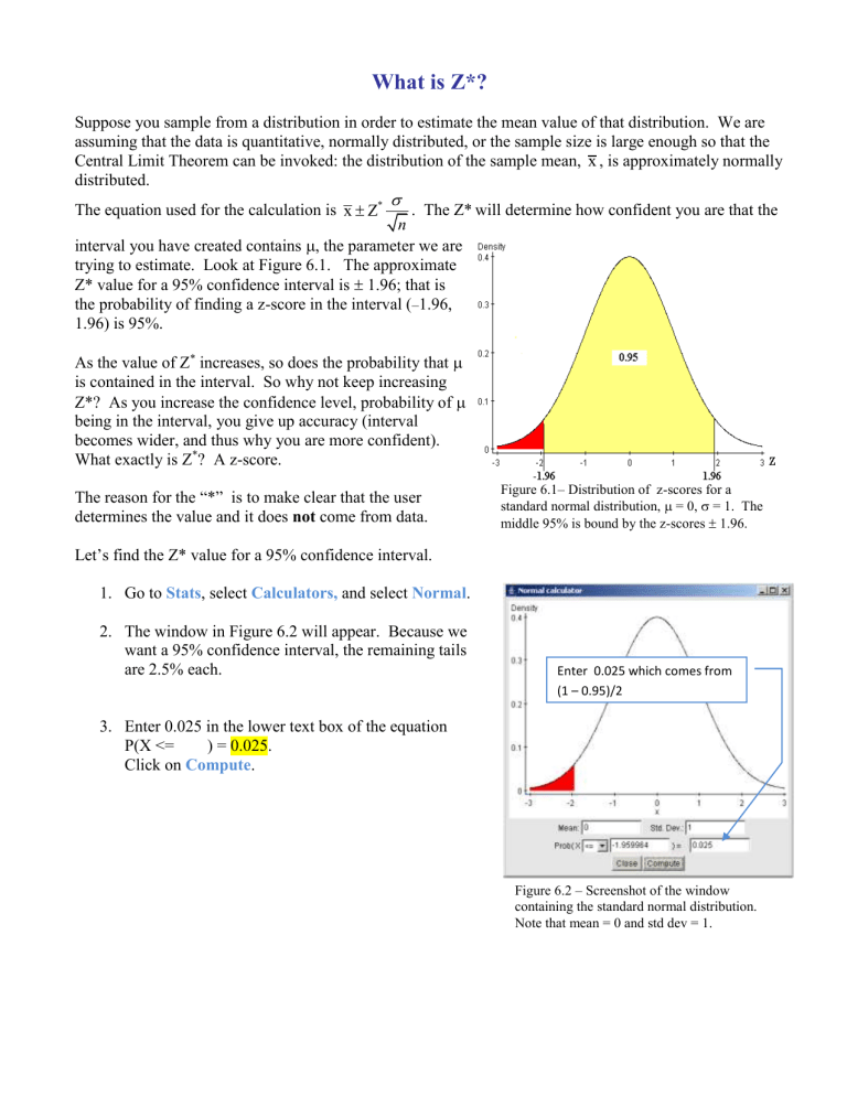
, the parameter we are trying to estimate. Look at Figure 6.1. The approximate
Z* value for a 95% confidence interval is

1.96; that is the probability of finding a z-score in the interval ( – 1.96,
1.96) is 95%.
As the value of Z
*
increases, so does the probability that
 is contained in the interval. So why not keep increasing
Z*? As you increase the confidence level, probability of
 being in the interval, you give up accuracy (interval becomes wider, and thus why you are more confident).
What exactly is Z
*
? A z-score.
The reason for the “*” is to make clear that the user determines the value and it does not come from data.
Let’s find the Z* value for a 95% confidence interval.
1.
Go to Stats , select Calculators , and select Normal .
2.
The window in Figure 6.2 will appear. Because we want a 95% confidence interval, the remaining tails are 2.5% each.
3.
Enter 0.025 in the lower text box of the equation
P(X <= ) = 0.025.
Click on Compute .
Figure 6.1– Distribution of z-scores for a standard normal distribution,

= 0,

= 1. The middle 95% is bound by the z-scores

1.96.
Enter 0.025 which comes from
(1 – 0.95)/2
Figure 6.2 – Screenshot of the window containing the standard normal distribution.
Note that mean = 0 and std dev = 1.