Linear Population Growth Model for Flour Beetles
Statement of Problem: The equations used to model the discrete population growth of
the flour beetle are given on page 39 of the text, equation 1.5.
Lt 1  bAt
Pt 1  Lt (1   L )
At 1  Pt (1   P )  At (1   A )
The parameter b is the birth rate of the species (number of Larvae produced each time
unit from an Adult). The parameters  L ,  P ,  A measure the death rates of the Larvae,
Pupae, and Adults, respectively.
We are asked to use Matlab to calculate the values for L, P, A for successive times given
initial conditions.
Note: Make sure you provide a thorough explanation of any mathematical material,
or modeling assumptions you have made.
Writeup: Because the model is linear, we expect exponential growth and/or decay to be
present. Using the Matlab code (linear_beetle.m) listed in Appendix 1, we used the same
values for b as for the nonlinear discrete model (equation 1.6 on page 40 of the text).
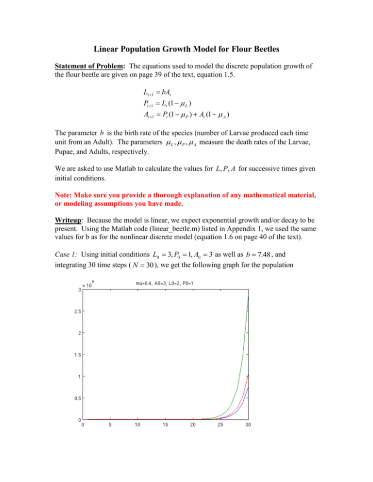
Case 1: Using initial conditions L0  3, P0  1, A0  3 as well as b  7.48 , and
integrating 30 time steps ( N  30 ), we get the following graph for the population
Note: Be sure to include lots of graphics. I have included one case study (for
illustrative purposes) but five to ten cases would be appropriate in this instance.
References: Any references (books, papers, web links) would go here …
Note: Web links should be given in full URL format (ie http://X.Y.Z/xyz). Journal
and book references should be complete, and in a consistent style.
Appendix 1 (Matlab Codes):
Listing for linear_beetle.m is given below
function linear_beetle(L0,A0,P0,N)
% Linear model for population growth
% Equations 1.5 on page 39 of text.
% The input arguments are initial conditions
% for L, A, P respectively
% Initialize static parameters ...
% to be those of the nonlinear model 1.6
b=7.48;
cea=0.009;
cel=0.012;
mul=0.267;
mup=0.0;
mua=0.4;
cpa=0.004;
% Create and initialize matrices ...
L=zeros(N,1);
P=zeros(N,1);
A=zeros(N,1);
% Set initial conditions ...
L(1)=L0;
A(1)=A0;
P(1)=P0;
% now, iteration N time steps ...
for i=1:N-1
L(i+1)=b*A(i);
P(i+1)=L(i)*(1-mul);
A(i+1)=P(i)*(1-mup)+A(i)*(1-mua);
end;
% Make a plot of the three dependent variables ...
t=1:N;
plot(t,A(t),t,L(t),t,P(t));
% Give it an informative title ...
title(sprintf('mu=%0.5g, A0=%0.5g, L0=%0.5g,
P0=%0.5g',mua,A(1),L(1),P(1)));
Note: Matlab listings should be formatted and commented!