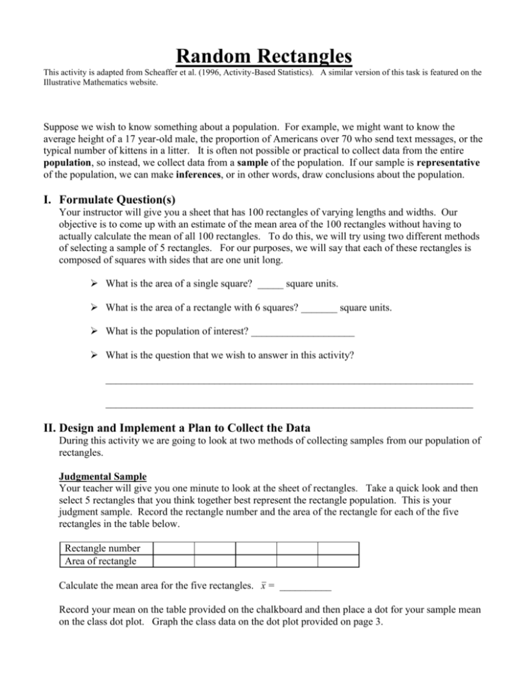
Random Rectangles
This activity is adapted from Scheaffer et al. (1996, Activity-Based Statistics). A similar version of this task is featured on the
Illustrative Mathematics website.
Suppose we wish to know something about a population. For example, we might want to know the
average height of a 17 year-old male, the proportion of Americans over 70 who send text messages, or the
typical number of kittens in a litter. It is often not possible or practical to collect data from the entire
population, so instead, we collect data from a sample of the population. If our sample is representative
of the population, we can make inferences, or in other words, draw conclusions about the population.
I. Formulate Question(s)
Your instructor will give you a sheet that has 100 rectangles of varying lengths and widths. Our
objective is to come up with an estimate of the mean area of the 100 rectangles without having to
actually calculate the mean of all 100 rectangles. To do this, we will try using two different methods
of selecting a sample of 5 rectangles. For our purposes, we will say that each of these rectangles is
composed of squares with sides that are one unit long.
 What is the area of a single square? _____ square units.
 What is the area of a rectangle with 6 squares? _______ square units.
 What is the population of interest? ____________________
 What is the question that we wish to answer in this activity?
_______________________________________________________________________
_______________________________________________________________________
II. Design and Implement a Plan to Collect the Data
During this activity we are going to look at two methods of collecting samples from our population of
rectangles.
Judgmental Sample
Your teacher will give you one minute to look at the sheet of rectangles. Take a quick look and then
select 5 rectangles that you think together best represent the rectangle population. This is your
judgment sample. Record the rectangle number and the area of the rectangle for each of the five
rectangles in the table below.
Rectangle number
Area of rectangle
Calculate the mean area for the five rectangles. x = __________
Record your mean on the table provided on the chalkboard and then place a dot for your sample mean
on the class dot plot. Graph the class data on the dot plot provided on page 3.
Simple Random Sample of Size 5
Now let’s take a simple random sample of 5 rectangles. We will use a random digits table to help us
randomly select rectangles. There are 100 rectangles. We will let 01 in the random digits table
correspond to rectangle 1, 02 to rectangle 2 and so on. Rectangle 100 will be represented by 00. First,
choose a starting row in the table. Select two digits at a time and record them in the table below. This
will correspond to the rectangles that will be sampled from your population of 100 rectangles. We are
sampling without replacement. (This means we do not want to select the same rectangle twice in the
same sample.) Skip over any repeated numbers.
Record the rectangle number and the area of the rectangle for each of the five rectangles in the table below.
Rectangle number
Size of rectangle
Calculate the mean area for the five rectangles. x = __________
Record your mean on the table provided on the chalkboard and then place a dot for your sample mean
on the class dot plot.
Repeat this process another four times: take four more samples of size 5, record the mean area of each
sample in the table below, record your means on the class table and then plot your value on the class
dot plot.
Sample
(n = 5)
Mean Area
1
2
3
4
5
Graph the class data on the dot plot provided on page 3.
Simple Random Sample of Size 10
Does sample size make a difference? Let’s take a simple random sample of 10 rectangles. Choose
another row in your random digits table and select 10 two-digit numbers. Find the mean area for the
10 identified rectangles and record
Sample
(n = 10)
Mean Area
1
2
3
4
5
Record your five means on the class table provided on the chalkboard and then place a dot for each of
your sample means on the class dot plot.
Graph the class data on the dot plot provided on page 3.
III. Analyzing the Data
Graph the class data for each of the three types of samples on the number lines provided below. Then
enter your data into a list in your calculator and use 1-Var Stats to find the mean and standard
deviation of the class sample means.
Judgment Sample
n = __________
mean of samples  x = ______
std dev of samples  x = ______
Judgment Sample
Simple Random Sample of Size 5
n = __________
mean of samples  x = ______
std dev of samples  x = ______
Simple Random Sample of Size 5
Simple Random Sample of Size 10
n = __________
mean of samples  x = ______
std dev of samples  x = ______
Simple Random Sample of Size 10
IV. Interpret the Results
A graph of the means of all the samples taken by the class is called a sampling distribution.
 Describe the shape, center and spread of each of the three sampling distributions.
Judgment Sample
Simple Random Sample of Size 5
Simple Random Sample of Size 10
 Decide which sampling method - judgmental sampling or simple random sampling - is the better
one for estimating the population mean, and explain your reasoning.
 How do the centers for the two sampling distributions taken with simple random samples of size 5
and size 10 compare?
 How do the shapes for the two sampling distributions taken with simple random samples of size 5
and size 10 compare?
 Look at the sampling distribution for simple random samples of size 10. How does its spread
compare to the spread of the sampling distribution for simple random samples of size 5?
 Ask your teacher for the actual mean size (area) of the population of 100 rectangles. How do the
centers of each sampling distribution compare to the population mean? Do any of the dot plots
have a center that is close to the mean area for the population of 100 rectangles?
Teacher Notes
New Illinois Learning Standards addressed by this activity:
Content Standards

Supporting
S
IC.1
This activity also lays the foundation for S.IC.4
and S.IC.5 mentioned at right.
Understand and evaluate random processes underlying statistical
experiments. Understand statistics as a process for making inferences
about population parameters based on a random sample from that
population.*
S.IC.4 Make inferences and justify conclusions from sample surveys,
experiments, and observational studies. Use data from a sample survey
to estimate a population mean or proportion; develop a margin of error
through the use of simulation models for random sampling.*
S.IC.5 Make inferences and justify conclusions from sample surveys,
experiments, and observational studies. Use data from a randomized
experiment to compare two treatments; use simulations to decide if
differences between parameters are significant.*
Primary Math Practices
MP 1 Make sense of problems and persevere in solving them.
MP 2 Reason abstractly and quantitatively.
MP 4 Model with mathematics.
MP 5 Use appropriate tools strategically.
MP 6 Attend to Precision.
MP 7 Look for and make use of structure.
Acknowledgements
This activity is adapted from Scheaffer et al. (1996, Activity-Based Statistics). A similar version of this task is
featured on the Illustrative Mathematics website.
The Simulation Process Model (SPM) handout was created by Sharon Lane-Getaz from St. Olaf College in
Minnesota. Additional information about using this handout as a tool to help students understand the
relationship between the population, samples of the population, and the sampling distribution can be found in
Using Simulation to Introduce Inference: An Active Learning Approach by Sharon Lane-Getaz and Andrew S.
Zieffler. (http://sharonlanegetaz.efoliomn.com/Uploads/Lane-Getaz,%20Zieffler%20JSM2006%2011-6-06.pdf)
Guidance for Class Activity
There are several key ideas that should be emphasized in this activity.
1) This activity includes the four components of statistical problem solving provided in the Guidelines for
Assessment and Instruction in Statistics Education (GAISE) Report. The four components are:
a. formulate a question
b. design and implement a plan to collect data
c. analyze the data by measures and graphs
d. interpret the results in the context of the original question.
2) Students should know the terms population and sample and be able to identify the population, the
sample and the sampling technique in a statistical study.
3) The opening paragraph introduces the idea that if our sample is representative we can make inferences
(draw conclusions) about the population. We select random samples as a means to insure that our
sample is not subject to bias and will therefore be representative of the population. In this activity, when
asked to select a judgmental sample of 5 rectangles that they feel are representative of the 100 rectangle
population, students tend to select samples that include more large rectangles and end up with an
average that is higher than the actual population mean. Our biases influence the rectangles that we
select.
4) Students tend to define random sampling as every observation in the population has an equal chance of
being selected. Students should learn that, while this is true to an extent, it is not a complete definition.
Selecting a random sample of size n actually means that all possible samples of size n from the population
has an equal chance of being selected. For example, if a class has 5 rows of 4 students, and the teacher
randomly selects a student from each row, then each student has an equal chance of being selected. This
is not, however, a simple random sample. Not all possible groups of size 5 had an equal chance of being
selected. The teacher has instead used stratified sampling – a sampling technique that can also be useful,
but is beyond the scope of what is covered in the New Illinois Learning Standards.
5) Students often confuse the relationship between a population, a sample and a sampling distribution.
Sharon Lane-Getaz, a professor at St. Olaf College in Minnesota, uses the Simulation Process Model (SPM)
as a tool for helping students see the relationship between the population, the samples, and the sampling
distribution. It is a great tool to use as part of the Random Rectangles activity as well as any other
simulation activity that you do with your students.
6) In statistics, our Roman alphabet is used to represent a sample statistic while the Greek alphabet is used
to represent population parameters. Begin to familiarize students with the letters that are used to
represent means and standard deviations for the following:
Population
Sample
Sampling Distribution

mean
proportion 
standard deviation 
sample mean x
sample proportion p
sample standard deviation s
mean of sample means  x
standard deviation of sample means  x
mean of sample proportions  p
standard deviation of sample means  p
7) Random Rectangles lays the ground work for the Central Limit Theorem which is covered in AP Statistics.
While students do not need to know the Central Limit Theorem, it is important for students to understand
some of the main ideas:
 The sampling distribution will be approximately normal if either the population distribution is
approximately normal or if the population is not unreasonably skewed and the sample size is
relatively large. (When sampling proportions, the population proportion is not too close to 0 or 1.)
 As the number of samples increases, the center of the distribution approaches the population
statistic being estimated (population mean, population proportion, population median, etc.).
 Larger sample sizes produce a sampling distribution with less spread. Smaller sample sizes
produce a sampling distribution with more spread.
8)
Answer Key
I. Formulate Question(s)
 What is the area of a single square? __1__ square unit.
 What is the area of a rectangle with 6 squares? __6____ square units.
 What is the population of interest? _The 100 rectangles on the Random Rectangle sheet._
 What is the question that we wish to answer in this activity?
___What is average (mean) area of the 100 rectangles?__________________________
_Or: What is the typical size (area) of a rectangle on this page?___________________
100 random samples of size 5
100 random samples of size 10
Dot Plot
Measures from Sample of Rectangles
2
4
6
8
10
Sam pleMean
12
14
2
16
4
mean
= 7.762
mean
= 7.67
count
= 100
count
= 100
stdDev
= 2.45438
stdDev
500 random samples of size 5
4
6
Dot Plot
12
14
16
8
10
Sam pleMean
12
14
Dot Plot
Measures from Sample of Rectangles
16
2
4
= 7.3564
mean
= 7.5814
count
= 500
count
= 500
= 2.39474
8
10
Sam pleMean
= 1.84826
mean
stdDev
6
500 random samples of size 10
Measures from Sample of Rectangles
2
Dot Plot
Measures from Sample of Rectangles
stdDev
= 1.71477
6
8
10
Sam pleMean
12
14
16
Population of 100 Rectangles (Population mean is 7.42 square units.)
Dot Plot
Rectangles
0
2
4
mean
= 7.42
count
= 100
stdDev
6
= 5.22848
8
10 12
Area
14
16
18
20