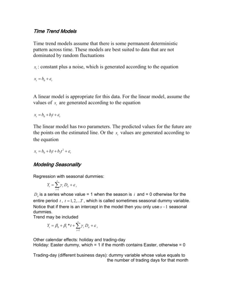
Time Trend Models
Time trend models assume that there is some permanent deterministic
pattern across time. These models are best suited to data that are not
dominated by random fluctuations
xt : constant plus a noise, which is generated according to the equation
xt  b0   t
A linear model is appropriate for this data. For the linear model, assume the
values of xt are generated according to the equation
xt  b0  b1t   t
The linear model has two parameters. The predicted values for the future are
the points on the estimated line. Or the xt values are generated according to
the equation
xt  b0  b1t  b2t 2   t
Modeling Seasonality
Regression with seasonal dummies:
s
Yt    i Dit   t
i 1
Dit is a series whose value = 1 when the season is i and = 0 otherwise for the
entire period t , t  1, 2,...T , which is called sometimes seasonal dummy variable.
Notice that if there is an intercept in the model then you only use s  1 seasonal
dummies.
Trend may be included
s
Yt   0  1 * t    i Dit   t
i 1
Other calendar effects: holiday and trading-day
Holiday: Easter dummy, which = 1 if the month contains Easter, otherwise = 0
Trading-day (different business days): dummy variable whose value equals to
the number of trading days for that month
Forecasting future values using the regression model.
Use SAS to show the data generating process and estimation.
SAS Program
data a;
retain date '01dec1990'd;
do i = 1 to 100;
date=intnx('month',date,1);
month=month(date);
year=year(date);
e1=rannor(1283) ;
if month=12 then do;
x=10+6+e1;
end;
else if month=1 then do;
x=10-5.5+e1;
end;
else do;
x=10+e1;
end;
output;
end;
run;
proc print;
id i year month;
var x;
run;
%macro PLOT(var,data);
goptions reset=global htitle=.5;
symbol1 interpol=join value=dot height=.1;
axis1 label=none;
axis2 label=none;
title1 "&var";
proc gplot data=&data;
plot &var*date/
haxis=axis1 vaxis=axis2;
run;
quit;
%mend;run;
%plot(x,a);
data b;
set a;
if month=12 then dum12=1;else dum12=0;
if month=1 then dum1=1;else dum1=0;
proc model;
endo x;
x=b0+b1*i+d1*dum1+d12*dum12;
fit;
run;
quit;
Exponential Smoothing Model
Exponential smoothing fits a time trend model using a smoothing scheme in
which the weights decline geometrically as you go backward in time. The
forecasts from exponential smoothing are a time trend, but the trend is based
mostly on the recent observations instead of on all the observations equally.
How well exponential smoothing works as a forecasting method depends on
choosing a good smoothing weight for the series.
Suppose X t is actual observations and Yt is smoothed series, t  1, 2,...n .
Assume:
Yt   X t   (1   ) X t 1   (1   )2 X t 2   (1   )3 X t 3  ....
(1)
where 0    1.
Notice that    (1   )   (1   )2  ....  1
To see that, let   (1   ) then
1     2   3  .... 
1




1
1 
1   1  (1   )
Since equation (1) is true for all t , it should hold true for t 1 .
Yt 1   X t 1   (1   ) X t 2   (1   )2 X t 3  ....
(2)
Multiplying (2) by (1   ) , we have
(1   )Yt 1   (1   ) X t 1   (1   )2 X t 2  ....
(3)
Subtracting equation (3) from (1) we have
Yt  (1   )Yt 1   xt
or
Yt   Xt  (1  )Yt 1
(4)
How to choose  ?
Define

et  X t  Yt 1 and S   et2
t 3
 should be chosen such that S is minimum.
It will yield constant forecasts for all future value of a time series, which is Yt .
(Excel Example)
Holt’s Linear Trend Algorithm
Yt   ( X t )  (1   )(Yt 1  Tt 1 )
Tt   (Yt  Yt 1 )  (1   )Tt 1
0  1
0   1
Yt and Tt are estimates of level and increment at time t , and  ,  are smoothing
constants.
How does it work?
At time t 1 , the latest estimates of level and slope are Yt 1 and Tt 1  a
new level Yt based on (Yt 1  Tt 1 ) for time t .
 and  are chosen to minimize one step ahead forecast errors.
(Excel Example)
Holt-Winters Algorithm for Seasonal Time Series
Yt , Tt and Ft are estimates of level, increment and season factor at time t , and
 ,  and  are smoothing constants.
Additive
Yt   ( X t  Ft S )  (1   )(Yt 1  Tt 1 )
0  1
Tt   (Yt  Yt 1 )  (1   )Tt 1
0   1
0  1
Ft   ( X t  Yt )  (1   )Ft S
If X t is monthly, S=12; if quarterly, S=4.
Multiplicative
Yt  
Yt
 (1   )(Yt 1  Tt 1 )
Ft s
Tt   (Yt  Yt 1 )  (1   )Tt 1
Xt
 (1   )Ft S
Yt
(Excel Example)
Ft  