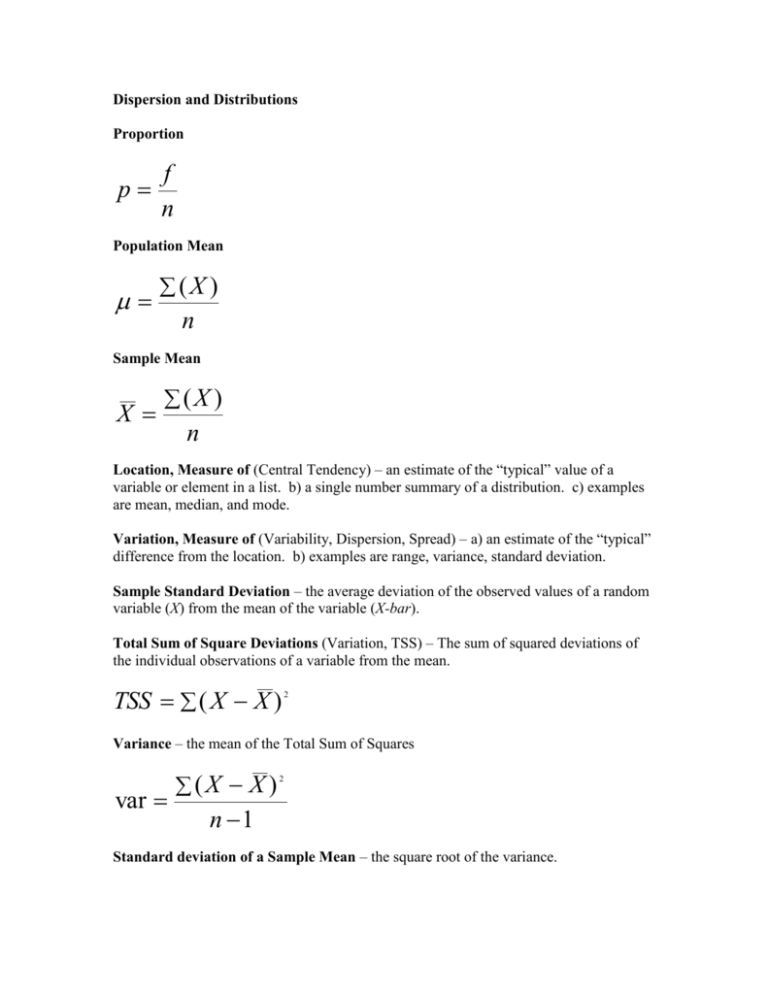
Dispersion and Distributions
Proportion
p
f
n
Population Mean

(X )
n
Sample Mean
X 
(X )
n
Location, Measure of (Central Tendency) – an estimate of the “typical” value of a
variable or element in a list. b) a single number summary of a distribution. c) examples
are mean, median, and mode.
Variation, Measure of (Variability, Dispersion, Spread) – a) an estimate of the “typical”
difference from the location. b) examples are range, variance, standard deviation.
Sample Standard Deviation – the average deviation of the observed values of a random
variable (X) from the mean of the variable (X-bar).
Total Sum of Square Deviations (Variation, TSS) – The sum of squared deviations of
the individual observations of a variable from the mean.
TSS   ( X  X )
2
Variance – the mean of the Total Sum of Squares
var 
(X  X )
2
n 1
Standard deviation of a Sample Mean – the square root of the variance.
sd 
(X  X )
2
n 1
Standard deviation of a Sample Proportion – the square root of the variance but
calculated as the square root of the probability (p) times the inverse of the probability
(q=1-p).
sd 
pq
Population Standard Deviation – a) the average deviation of the population values of a
random variable (X) from the mean of the variable (μ). b)like other population
parameters is generally not known or observable. c) symoblied as sigma, like other
population parameters a Greek letter.

 (X  )
2
N
Normal Probability Distribution (Normal Curve, Gaussian Distribution, Bell Curve) –
a) a bell shaped continuous probability distribution that describes data that cluster around
the mean. b) is used as a simple model of complex phenomenon and is the basis of many
inferential statistics. c) 68% of the observations are within one standard deviation of the
mean, 5% of the observations are more than 1.96 standard deviations from the mean and
10% are more than 1.64 standard deviations from the mean. d) was formalized by Johann
Carl Friedrich Gauss (1777-1855), a German mathematician, although he was not the first
to conceptualize it.
x  N (  ,  ) 
Law of Large Numbers – a) in probability theory, a theorem that states that the average
of the results obtained from a large number of trials should be close to the expected
value. b) the mean from a large number of samples should be close to the population
mean. c) the first fundamental theorem of probability.
Central Limit Theorem – a) in probability theory, a theorem that states that the mean of
a sufficiently large number of independent random trials, under certain common
conditions, will be approximately normally distributed. b) as the sample size increases
the distribution of the sample means approaches the normal distribution irrespective of
the shape of the distribution of the variable. c) from a practical standpoint, many
distributions can be approximated by the normal distribution, including the binomial
(coin toss), Poisson (event counts), and Chi-Squared. d) justifies the approximation of
large-sample statistics to the normal distribution. e) the first fundamental theorem of
probability.
Sampling Distribution – a) the distribution of a statistic, like a mean, for all possible
samples of a given size. b) based on the law of large numbers and the central limit
theorem, the sampling distribution will have a mean equal to the population mean and
will be normally distributed.
Standard Normal Probability Distribution (Z-distribution) – a) a normal probability
distribution with mean 0 and variance/standard deviation 1. b) any other normal
distribution can be regarded as a version of the standard normal distribution that has been
shifted rightward or leftward to center on the actual mean and then stretched horizontally
by a factor the standard deviation.
x  N (0,1)
Z-Scores (Normal Deviates) – a standardized score that converts a variable (x) into a
standard normal distribution with mean = 0 and sd =1 and a metric of standard deviations
from the mean.
X X
z
sd
X  ( z * sd )  X
Student’s t-distribution – a) a probability distribution used for estimating the mean of a
normally distributed population when the sample size is small, that is 50 or less. b) the
overall shape of the t-distribution resembles the bell shape of the z-distribution with a
mean of 0 and a standard deviation of 1, except that it is a bit lower at the peak with fatter
tails. c) as the sample size increases, that is the number of degrees of freedom increase,
the t-distribution more and more closely approximates the normal distribution, that is it
asymptotically approaches normality. d) can be thought of not as a single distribution,
like the z-distribution, but a family of distributions that vary according to the sample size,
that is degrees of freedom. e) at a sample size of 50 (that is 49 degrees of freedom), 5%
of the observations are more than 2.009 standard deviations from the mean (compared to
1.96 in the normal distribution) and 10% are more than 1.676 standard deviations from
the mean (compared to 1.64 in the normal distribution).f) is generally the distribution
used in estimating confidence intervals and inferential tests of the difference between
sample means and sample means and hypothesized population means, instead of the zdistribution. g) was developed by William Sealy Gosset in his research aimed at
selecting the most productive and consistent varieties of barley for brewing beer and was
first published in 1908 using the pseudonym “Student” because his employer, the
Guinness Brewery in Dublin, Ireland, prohibited its employees from publishing scientific
research due to a previous disclosure of trade secrets by another employee.
Standard Error - a) the standard deviation of a sampling distribution. b) a probabilistic
estimate of the sampling error representing the spread or dispersion of the sample
estimates. c) the part of the standard deviation of a variable that can be attributed to
sampling variability, that is sampling error.
se 
sd
n