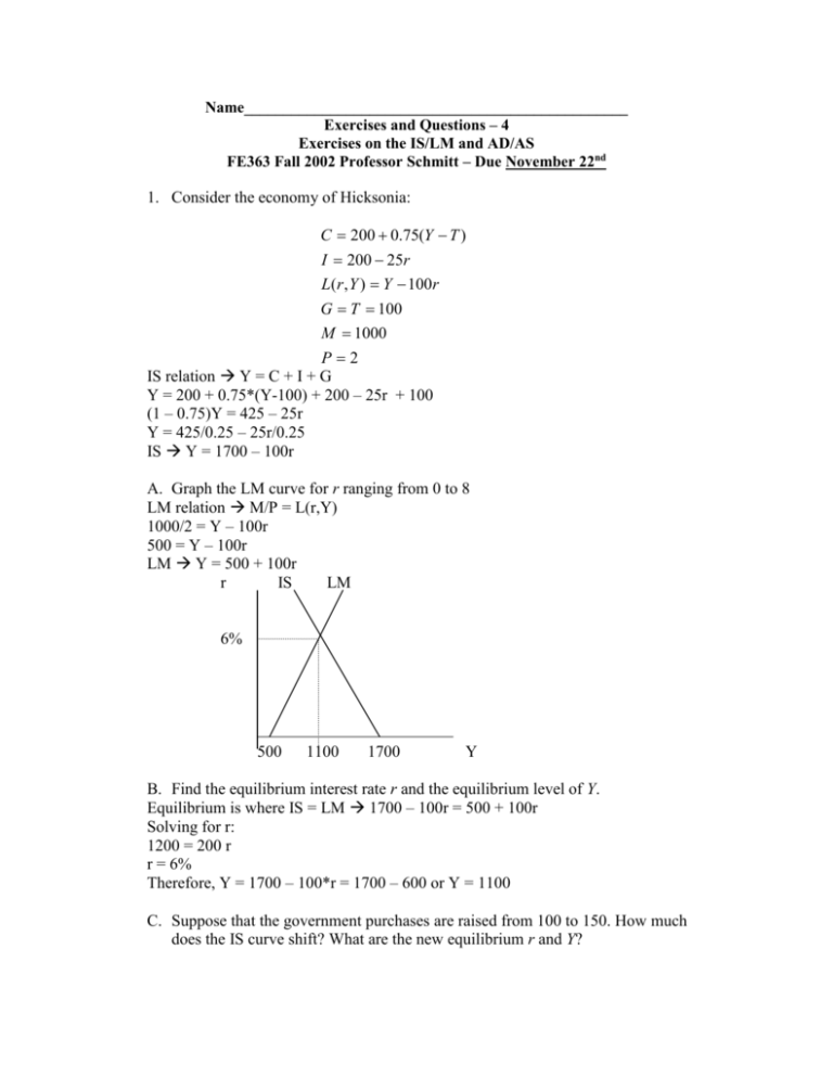
Name_________________________________________________
Exercises and Questions – 4
Exercises on the IS/LM and AD/AS
FE363 Fall 2002 Professor Schmitt – Due November 22nd
1. Consider the economy of Hicksonia:
C  200  0.75(Y  T )
I  200  25r
L(r , Y )  Y  100r
G  T  100
M  1000
P2
IS relation  Y = C + I + G
Y = 200 + 0.75*(Y-100) + 200 – 25r + 100
(1 – 0.75)Y = 425 – 25r
Y = 425/0.25 – 25r/0.25
IS  Y = 1700 – 100r
A. Graph the LM curve for r ranging from 0 to 8
LM relation  M/P = L(r,Y)
1000/2 = Y – 100r
500 = Y – 100r
LM  Y = 500 + 100r
r
IS
LM
6%
500
1100
1700
Y
B. Find the equilibrium interest rate r and the equilibrium level of Y.
Equilibrium is where IS = LM  1700 – 100r = 500 + 100r
Solving for r:
1200 = 200 r
r = 6%
Therefore, Y = 1700 – 100*r = 1700 – 600 or Y = 1100
C. Suppose that the government purchases are raised from 100 to 150. How much
does the IS curve shift? What are the new equilibrium r and Y?
If G  to 150
Y = C + I + G  so Y = 200 + 0.75(Y-100) + 200 – 25r + 150
Y = 1900 – 100r
Note you could also have determined that
G = 50 so Y = (1/(1-mpc))*G = 4*50 = 200
r
IS1 IS2 LM
7%
6%
500
1100
1700
Y
1200
To find the equilibrium set the IS relation = LM relation
1900 – 100r = 500 + 100r
1400 = 200r
r = 7%
Y = 1900 – 100*r = 1200
D. With the initial value for fiscal policy (G =100), suppose the price level rises from
2 to 4. What happens? What are the new equilibrium interest rate and level of
income?
This will change real money balances
LM relation  M/P = L(r,Y)
1000/4 = Y – 100r
250 = Y – 100r
LM  Y = 250 + 100r
r
IS
LM2 LM1
7.25%
6%
250 500 1100 1700
975
r = 7.25% and Y = 975 (follow same math steps)
Y
E. Derive and graph an equation for the aggregate demand curve. What happens to
this aggregate demand curve with the fiscal policy mentioned in part D?
AD is the relationship between the price level and the level of income. Therefore we
need to substitute out for the interest rate. To do this solve for the the IS and LM for
the interest rate:
IS: Y =1,700 – 100r
LM: M/P = Y – 100r
Price Levels
So we can solve for 100r:
IS  100r = 1,700 – Y
LM  100r = Y – M/P
Setting these equal:
1,700 – Y = Y – M/P
2Y = 1700 + M/P
Y = 850 + M/2P
AD = 850+500/P
Y – output
Since M = 1000 this is Y = 850 + 500/P
I derived AD for part D. If I derived for parts A and B then the increase in G would
shift AD to the right.
2. In a small open economy – if a domestic country does not want to change net
exports, but wants to stimulate their economy, according to the Mundell-Fleming
model, what combinations of monetary and fiscal policy should you pursue? Hint:
You will need to make a few assumptions to answer this question – state them
clearly. Illustrate with a graph.
To keep NX constant and increase Y, a 1) small open economy, with 2) perfect
capital mobility, and with 3) fixed exchange rates (“pegging”)
Needs to engage in expansionary fiscal policy.
r
LM1
LM2
r*1
(1) 
IS1
Y1
 G or  T  IS1  IS2
This puts upward pressure on r .
As r > r* capital flows in and e 
Peg 100Y/$1 pressure to 150Y/$1
Y2
IS2
Y
 market is selling Yen and buying dollars
 Fed sells dollars and buys yen. Fed sells domestic currency and sells foreign
currency.
  M  (M/P)   LM1  LM2
 (M/P)  r  and removes incentives for capital flow.
Result: Under a fixed exchange rate, fiscal expansion is effective in  Y under perfect
capital mobility.
3. Suppose you wanted to make domestic industries more competitive, but did not
want to alter aggregate income. According to the Mundell-Fleming model, what
combinations of monetary and fiscal policy should you pursue – and what
assumptions do you have to make regarding exchange rates?
To decrease M and/or increase X (making domestic industry more competitive) – NX
would  while keeping constant Y, a 1) small open economy, with 2) perfect capital
mobility, and with 3) floating exchange rates
Needs to engage in contractionar fiscal policy.
4. Using the following data, interpret the situation on an IS-LM curve. One clear
thing during this time period, the great depression, is that C fell (arguably due to
the stock market crash and consumer confidence) and also I fell (arguably due to
decreased housing needs of immigrants).
A. Graph the IS/LM model with the fall in C and I.
r
IS2 IS1
LM
r1
r2
Y2 Y1
B. State the Fiscal and/or Monetary Policy changes – and show on the
previous graph the shift in IS and/or LM. Focus specifically on the policy
changes from 1931 to 1993 ONLY.
In 1931 to 1933 – there was fiscal AND monetary contraction: G and M
r
IS2 IS1 LM2 LM1
r1
Y2
Y1
Expect interest rates to return, but output to fall even further than in A.
C. Do the data match your predictions for short-run changes in
unemployment, income, and interest rates?
Predict that with Y   U  and r return to 1931 rates
This is true for Y and U, but r does not return, in fact r  further!
D. Did either policy help the recession?
Nope – may have had it extend
E. If the policies implemented in 1931 – 1933 continued in the same
direction – would the economy ever recover – or did recovery only occur
due to the Fiscal and/or Monetary Policies implemented after 1933?
Can’t say for sure – in the long-run we should see that U causes price levels
to fall (as workers will now work for less). This does happen to some degree –
which should increase the SRAS and increase the LM…
Year GDPR
1929
1930
1931
1932
1933
1934
1935
1936
1937
1938
1939
1940
UR
C
I
G
RB
M1
P(58$)
Real
GDP
Unemp
rate
Consumption
Investment
Government
Purchases
Interest
rates
Money
supply
Price
level
203.6
183.5
169.5
144.2
141.5
154.3
169.5
193.2
203.2
192.9
209.4
227.2
3.2
8.9
16.3
24.1
25.2
22.0
20.3
17.0
14.3
19.1
17.2
14.6
139.6
130.4
126.1
114.8
112.8
118.1
125.5
138.4
143.1
140.2
148.2
155.7
40.4
27.4
16.8
4.7
5.3
9.4
18.0
24.0
29.9
17.0
24.7
33.0
22.0
24.3
25.4
24.2
23.3
26.6
27.0
31.8
30.8
33.9
35.2
36.4
5.9
3.6
2.6
2.7
1.7
1.0
0.8
0.8
0.9
0.8
0.6
0.6
26.6
25.8
24.1
21.1
19.9
21.9
25.9
29.6
30.9
30.5
34.2
39.7
50.6
49.3
44.8
40.2
39.3
42.2
42.6
42.7
44.5
43.9
43.2
43.9