Lecture Notes
AMS312 Spring207
Mar 6th
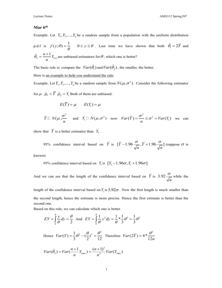
Example: Let Y1 , Y2 ,..., Yn be a random sample from a population with the uniform distribution
p.d.f is
ˆ2 
f ( y;  ) 
1
0  y   . Last time we have shown that both ˆ1  2Y and

n 1
Y( n ) are unbiased estimators for  , which one is better?
n
The basic rule is: compare the Var (ˆ1 ) and Var (ˆ2 ) , the smaller, the better.
Here is an example to help you understand the rule:
Example: Let Y1 , Y2 ,..., Yn be a random sample from N (  ,  ) . Consider the following estimator
2
for  . ˆ1  Y ˆ 2  Y1 Both of them are unbiased:
E (Y )  
Y
2
N ( ,
n
E (Y1 )  
) and Y1
N (  ,  2 ) now Var (Y ) 
2
n
  2  Var (Y1 ) we can
show that Y is a better estimator than Y1 .
95% confidence interval based on Y is [Y  1.96

n
, Y  1.96

n
] (suppose  is
known)
95% confidence interval based on Y1 is [Y1  1.96 , Y1  1.96 ]
And we can see that the length of the confidence interval based on Y is 3.92

n
while the
length of the confidence interval based on Y1 is 3.92 . Now the first length is much smaller than
the second length, hence the estimate is more precise. Hence the first estimate is better than the
second one.
Based on this rule, we can calculate which one is better.

EY  
0
y

dy 

2

And EY  
0
1

y 2 dy 
1 1 3 1 2
*   
 3
3
1 2  2 2
2
Hence Var (Y )    ( ) 
Therefore Var (2Y )  4*
3
2
12
12n
Var (ˆ2 )  Var (
n 1
(n  1) 2
Ymax ) 
Var (Ymax )
n
n2
1
Lecture Notes
AMS312 Spring207
y
FY( n ) ( y )  P(Y( n )  y )  P(max{Y1 , Y2 ,..., Yn }  y )   P(Yi  y )  ( ) n

fY( n ) ( y) 
d
ny n1
FY( n ) ( y)  n
dy


E (Y( n ) 2 )  
0

E (Y( n ) )  
0
ny n 1
n
ny n 1

n
y 2 dy 
ydy 
Therefore, Var (Y( n ) ) 
n n
n 2

n n2 n2
n

n 1
n 2
n
2
(
 )2 
n  2 n 1
n(n  2)
Now we see that Var (ˆ1 )  Var (ˆ2 ) hence ˆ2 is a better estimator.
If we define 3  2Y1 then E (2Y1 )  
and Var (2Y1 )  4Var (Y1 ) 
2
3
. It is bigger
than Var (ˆ1 ) .
If we define ˆ4 
ˆ1  ˆ2
2
hence E (ˆ4 )   the variance is between the variance of ˆ1 and the
variance of ˆ2 .
Var (ˆ1 ) n  2
The efficiency of ˆ2 in relative of ˆ1 is

Var (ˆ2 )
3
Also study ex5.4.6 in page 389.
Section5.5 Minimum—variance estimators. The C-R Lower bound.
Theorem: Let Y1 , Y2 ,..., Yn be a random sample from the continuous pdf fY ( y; ) , where
fY ( y; ) has continuous first-order and second-order partial derivatives at all but a finite set of
points. Suppose that the set of ys for which
fY ( y; )  0 does not depend on  . Let
ˆ  h(Y1, Y2 ,..., Yn ) be any unbiased estimator for  .Then
Var (ˆ)  {nE[(
 ln fY ( y; ) 2 1
 2 ln fY ( y; ) 1
) ]}  {nE[
]}

 2
(A similar statement holds if the n observations come from a discrete pdf, p X (k ; ) )
2
Lecture Notes
AMS312 Spring207
Example: f ( y; ) 
1

0  y   cannot apply the Cramer-Rao lower bound.
Example: If Y1 , Y2 ,..., Yn is random sample for N (  ,  )
2
1 
Population pdf: fY ( y;  ,  ) 
e
2
2
( y   )2
 y  
2 2
For the estimator of  : ˆ1  Y (MLE and MOME)
ˆ 2  Y1 , ˆ3 
Y  Y2  ...  Yn 1
Y1  Y
, ˆ 4  1
n 1
2
Now we calculate the Cramer-Rao lower bound:

1
ln fY ( y;  ,  )  ln[
e
2
( y   )2
2
2 2
]   ln( 2 ) 
( y   )2
2 2
 2 ln fY ( y;  ,  2 )  y  
1

[ 2 ] 2
2

 

E ( ˆ )   and Var ( ˆ )  n[ E (
1
2

n
)]1 
2
Definition (Best estimator (minimum variance estimator for  )):
Let  be an unbiased estimator for  if Var (  )  Var (  ) where  is any unbiased estimator
*
*
for  .  is called the best estimator for  .
*
Definition (Efficient estimator for  ): If Var ( ˆ ) reaches the Cramer-Rao Lower Bound,
then ̂ is called the efficient estimator for  .
3