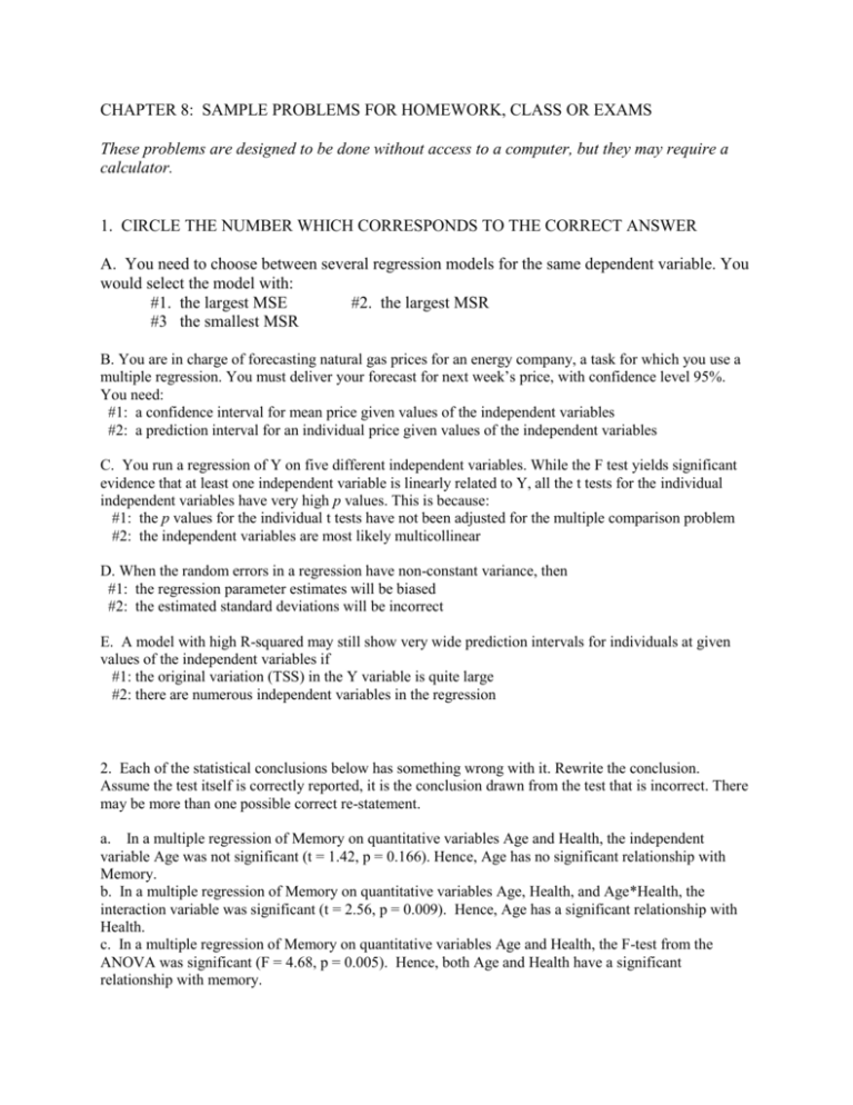
CHAPTER 8: SAMPLE PROBLEMS FOR HOMEWORK, CLASS OR EXAMS
These problems are designed to be done without access to a computer, but they may require a
calculator.
1. CIRCLE THE NUMBER WHICH CORRESPONDS TO THE CORRECT ANSWER
A. You need to choose between several regression models for the same dependent variable. You
would select the model with:
#1. the largest MSE
#2. the largest MSR
#3 the smallest MSR
B. You are in charge of forecasting natural gas prices for an energy company, a task for which you use a
multiple regression. You must deliver your forecast for next week’s price, with confidence level 95%.
You need:
#1: a confidence interval for mean price given values of the independent variables
#2: a prediction interval for an individual price given values of the independent variables
C. You run a regression of Y on five different independent variables. While the F test yields significant
evidence that at least one independent variable is linearly related to Y, all the t tests for the individual
independent variables have very high p values. This is because:
#1: the p values for the individual t tests have not been adjusted for the multiple comparison problem
#2: the independent variables are most likely multicollinear
D. When the random errors in a regression have non-constant variance, then
#1: the regression parameter estimates will be biased
#2: the estimated standard deviations will be incorrect
E. A model with high R-squared may still show very wide prediction intervals for individuals at given
values of the independent variables if
#1: the original variation (TSS) in the Y variable is quite large
#2: there are numerous independent variables in the regression
2. Each of the statistical conclusions below has something wrong with it. Rewrite the conclusion.
Assume the test itself is correctly reported, it is the conclusion drawn from the test that is incorrect. There
may be more than one possible correct re-statement.
a. In a multiple regression of Memory on quantitative variables Age and Health, the independent
variable Age was not significant (t = 1.42, p = 0.166). Hence, Age has no significant relationship with
Memory.
b. In a multiple regression of Memory on quantitative variables Age, Health, and Age*Health, the
interaction variable was significant (t = 2.56, p = 0.009). Hence, Age has a significant relationship with
Health.
c. In a multiple regression of Memory on quantitative variables Age and Health, the F-test from the
ANOVA was significant (F = 4.68, p = 0.005). Hence, both Age and Health have a significant
relationship with memory.
3. A researcher has collected data on log(Income) for 600 men in Jacksonville. Log(Income) is
used as the independent variable in a series of multiple regressions using independent variables
X1 = Age in years
X2 = Years of Education
X3 = Race (0=white/1=nonwhite) .
The full model has SSE(Int, X1, X2, X3, X1*X2, X1*X3, X2*X3) = 35.38.
Various simpler models had
SSE(Int, X1, X2, X3) = 35.90
SSE(Int, X1, X3, X1*X3) = 36.09
SSE(Int, X2, X3, X2*X3) = 49.85
SSE(Int) = 66.10
Int is short for Intercept, that is, 0 .
a. What is R-squared for the full model?
b. Test the null hypothesis that X2 has no association of any kind (either alone or through an
interaction). Use  = 5%.
4. You are carry out a regression of child’s Reading Score on the independent variables AGE
(in years), MOM (Mother’s years of formal education), INCOME (household income in $1000s).
Part of the regression printout is summarized below. There were 200 children in the sample.
Variable
Parameter Estimate
Standard Error
Intercept
-29.4
6.32
AGE
8.56
1.68
MOM
1.24
.35
INCOME
.28
.095
a. Give a 95% confidence interval for the increase in mean reading scores if INCOME increases
by 10 ($10,000), if AGE and MOM’s education are held constant.
b. Previous research had indicated that mean reading scores increased by 10 points for each
additional year of AGE, provided other independent variables are held constant. Does this data
provide evidence to dispute that claim? Use  = 10%.
5. An urban planner is studying Y = per capita property tax base for various neighborhoods (in
$1000s) as a function of X1 = average age of homes and X2 = average size of homes. Data are
available for a sample of 120 neighborhoods, in which TSS = 17,136. Here is information on
two models.
Model 1: y  0  1X1  2X2  3X1X2  , R2  0.365
Model 2: y  0  2X2  , R2  0.303
Does Model 1 fit significantly better than Model 2, assuming  = 5%? What does your result
imply regarding the association with age of homes?
6. You are modeling the Hardness of polyester resins as a function of X1 = curing time. Several
models are fit using polynomials in X1. Based on the SSE given below, what order polynomial
would you recommend for use as a model? There were 20 observations in the data.
TSS = 76
SSE from linear model = 42
SSE from quadratic model = 28
SSE from cubic model = 24
SSE from quartic model = 22
7. The effect of extra tutoring hours (X1) on math scores (Y) is being studied in high-risk High
School students. We also want to control for each student’s hours per week outside class spent
studying on their own (X2). Our primary emphasis is on studying the effect of X1.
The regression printout is attached.
a. Using the graph on the next page, plot the predicted value for Y when X2 = 0 and again when
X2 = 8. Note that some of the predicted values have already been computed for you:
when X1 = 0 and X2 = 0, then Yˆ = 25.4
when X1 = 3 and X2 = 0, then Yˆ = 31.0
when X1 = 0 and X2 = 8, then Yˆ = ________?
when X1 = 3 and X2 = 8, then Yˆ = 63.6
b. Using your graph as a guide, explain in terms that a non-statistician can understand how extra
tutoring hours (X1) affects expected math scores. Under what conditions is the extra tutoring
most helpful?
c. Give a 95% confidence interval for the increase in mean math scores if tutoring hours are
increased by 1, AND hours spent studying on their own (X2) is held at 0.
PRINTOUT FOR PROBLEM 7
Number of Observations Used
80
Analysis of Variance
Source
DF
Sum of
Squares
Mean
Square
Model
Error
Corrected Total
3
76
79
6210.08235
8543.05152
14753
2070.02745
112.40857
Root MSE
Dependent Mean
Coeff Var
10.60229
41.36909
25.62853
R-Square
Adj R-Sq
F Value
Pr > F
18.42
<.0001
0.4209
0.3981
Parameter Estimates
Variable
Intercept
x1
x2
x1x2
DF
1
1
1
1
Parameter
Estimate
25.39257
1.85587
1.93391
0.71724
Standard
Error
4.52073
2.56473
0.87829
0.52000
t Value
5.62
0.72
2.20
1.38
Pr > |t|
<.0001
0.4715
0.0307
0.1718
Variance
Inflation
0
5.85170
3.07128
7.49525
80
70
60
50
40
30
20
10
0
1
X1
=
2
ext r a
hour s
of
t ut or i ng
3
8. In an agricultural experiment, the dependent variable YIELD = 10s of pounds of tomatoes per
1000 sq ft of plantings is modeled using on FERTILZ = 10s of pounds of fertilizer per 1000 sq
ft, SPRGRAIN = spring rainfall in centimeters. The attached regression printout shows the
results of regressing Yield on FERTILZ, SPRGRAIN and the interaction
SPRGFERT=SPRGRAIN*FERTILZ. The focus of our study is the effect of Fertilizer
a. Draw a plot of expected Yield versus Fertilz when Sprgrain = 10 inches, and also when
Sprgrain = 30 inches. You may superimpose your plot on the scatterplot below. Values of
Fertilz ranged from 2 to 7. See fitted values already computed below.
TO Help you, some of the fitted values have already been computed
When SprgRain=10
and Fertilz=2 Estimated Yield = 561
SprgRain=30
and Fertilz=2
Estimated Yield = 683
SprgRain=10
and Fertilz=7
Estimated Yield = 723
SprgRain=30
and Fertilz=7
Estimated Yield = _____ ?
1100
1000
900
800
700
600
500
2
3
4
Fer t i l i z er
5
i n
10s
of
6
7
pounds
b. Using your plot, describe the effect of Fertilizer. Is Fertilizer more effective when spring
rains are heavy or when they are light?
c. Is there significant evidence, at  = 5%, that at least one of the independent variables is
related to Yield? Cite the appropriate test statistic and its p-value.
d. Is there significant evidence, at  = 5%, that adding the interaction term to a model that has
SprgRain and Fertilz will improve prediction of yields? Cite the appropriate test statistic and its
p-value.
e. Discuss the reasonableness of the regression assumptions, citing the available evidence.
PRINTOUT FOR PROBLEM 8
Number of Observations Used
93
Analysis of Variance
DF
3
89
92
Sum of
Squares
805740
7127.05286
812867
Root MSE
Dependent Mean
Coeff Var
8.94870
734.46929
1.21839
Source
Model
Error
Corrected Total
Variable
Intercept
fertilz
sprgrain
sprgfert
DF
1
1
1
1
Parameter
Estimate
475.28935
11.93061
2.04230
2.04754
Mean
Square
268580
80.07925
R-Square
Adj R-Sq
F Value
3353.93
0.9912
0.9909
Parameter Estimates
Standard
Error
t Value
12.30734
38.62
2.68275
4.45
0.61353
3.33
0.13299
15.40
Variance
Inflation
0
17.13569
9.82387
26.56513
Pr > |t|
<.0001
<.0001
0.0013
<.0001
Plot of Residuals versus predicted values
30
20
10
0
- 10
- 20
- 30
500
600
700
800
pr edi ct ed
900
yi el d
Pr > F
<.0001
1000
1100
SOLUTIONS
1 a. #2
b. #2
c. #2
d. #2
e. #1
2 a. There is no significant evidence that Age is related to Memory, provided Health is kept
constant.
b. There is significant evidence that the relation of Age with Memory varies by value of Health.
OR There is significant evidence that the relation of Health with Memory varies by value of Age.
c. There is significant evidence that at least one of Health or Age have a relationship with
Memory.
3. a. R-squared = (66.1 – 35.38) / 66.1 = 0.465
b.
36.09  35.38
(596  593)
F 
 3.97
35.38 / 593
with 3 and 593 df. The critical value is 2.60. There is
significant evidence that X2 has some type of association with ln(Income).
4. a. 10 0.28  1.96 * 0.095  (0.94,4.66)
With confidence 95%, if income increases by 10 units, then the expected increase in reading
score is between 0.94 and 4.66 units.
b. Ho: age  10 . t 
8.56  10
 0.857 with 196 df. There is no significant evidence that
1.68
the claim is incorrect.
5. For model 1, SSE = (1-0.365)*17136 = 10881.36 with 114 df
For model 2, SSE = (1 – 0.303)*17136 = 11943.792 with 116 df
F = 5.66 with 2 and 114 df. There is significant evidence that average age has some type of
association with per capita property tax base.
6. The MSE from the full quartic model is 22/(20-5) = 1.467. The sequential sums of squares,
beginning with a model that only has an intercept, would be
Source
SS
F
Linear
76-42 = 34
23.18
Quadratic
42-28 = 14
9.54
Cubic
28-24 = 4
2.73
Quartic
24-22 = 2
1.36
The critical value with 1 and 15 df is 4.54. This suggests that a quadratic model would fit the
data adequately.
7. a. When X1=0 and X2=8, then Yˆ =40.86
b. The dashed line shows the relation of
Y with X1 when X2 (time outside class)
is 0. The solid line is when X2 is 8.
Extra tutoring only has a small impact
on expected scores when the student
does not spend any extra hours outside
of class. However, if the student does
spend extra hours outside of class, the
tutoring is associated with a great
increase in scores.
c. This is a confidence interval for 1 .
1.85591.9921(2.5647) = (-3.25,6.97)
When there is no extra time outside
class, the tutoring does not have any
significant effect.
8. a. When Sprgrain=30 and
Fertilz=7, predicted yield is 1050
b. The graph shows that increasing
Fertilizer is always associated with
increasing levels of yield, but that the
impact of increasing fertilizer is
stronger when there is greater spring
rain.
c. F = 3353.93, p < 0.0001, there is
extremely strong evidence that at least
one of the independent variables is
associated with yields.
d. t = 15.4, p < 0.0001, yes there is
significant evidence that adding an
interaction to the model that has Sprgrain and Fertilz will improve prediction.
e. The residual plot does not show any crescent shape, that is, no sign of nonlinearity, nor any
flare, that is no sign of nonconstant variance. There are no obvious outliers.