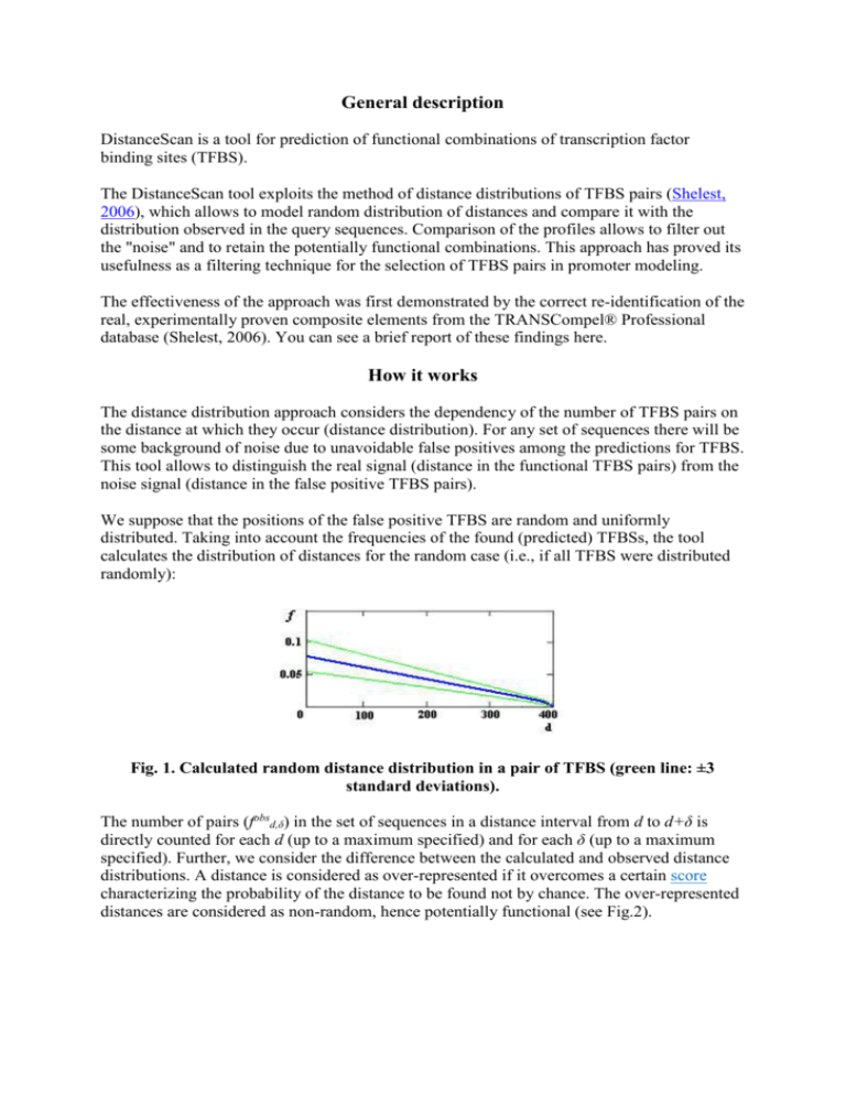
General description
DistanceScan is a tool for prediction of functional combinations of transcription factor
binding sites (TFBS).
The DistanceScan tool exploits the method of distance distributions of TFBS pairs (Shelest,
2006), which allows to model random distribution of distances and compare it with the
distribution observed in the query sequences. Comparison of the profiles allows to filter out
the "noise" and to retain the potentially functional combinations. This approach has proved its
usefulness as a filtering technique for the selection of TFBS pairs in promoter modeling.
The effectiveness of the approach was first demonstrated by the correct re-identification of the
real, experimentally proven composite elements from the TRANSCompel® Professional
database (Shelest, 2006). You can see a brief report of these findings here.
How it works
The distance distribution approach considers the dependency of the number of TFBS pairs on
the distance at which they occur (distance distribution). For any set of sequences there will be
some background of noise due to unavoidable false positives among the predictions for TFBS.
This tool allows to distinguish the real signal (distance in the functional TFBS pairs) from the
noise signal (distance in the false positive TFBS pairs).
We suppose that the positions of the false positive TFBS are random and uniformly
distributed. Taking into account the frequencies of the found (predicted) TFBSs, the tool
calculates the distribution of distances for the random case (i.e., if all TFBS were distributed
randomly):
Fig. 1. Calculated random distance distribution in a pair of TFBS (green line: ±3
standard deviations).
The number of pairs (fobsd,δ) in the set of sequences in a distance interval from d to d+δ is
directly counted for each d (up to a maximum specified) and for each δ (up to a maximum
specified). Further, we consider the difference between the calculated and observed distance
distributions. A distance is considered as over-represented if it overcomes a certain score
characterizing the probability of the distance to be found not by chance. The over-represented
distances are considered as non-random, hence potentially functional (see Fig.2).
Fig. 2. The distribution of distances in a set of sequences containing known composite
elements (red line) compared with the random distance distribution calculated for the
same set (blue line). The green line shows the score corresponding to the p-value~0.05.
The workflow includes 4 main steps:
 Identification of pairs;
 Measuring the number of pairs in a distance interval;
 Calculation of random distance distributions for the sequence sets;
 Selection of the over-represented peaks.
Presently DistanceScan is working with 3 kinds of inputs: (i) the results of a PWM-based
TFBS prediction (MatchTM output), (ii) the results of motif prediction (Gibbs Sampler output),
and (iii) the results of two-step prediction of motifs and corresponding PWM search
(MEME/FIMO output).
How to start
1. Select the input format.
Presently there are 3 formats taken as an input by DistanceScan: the output of the MatchTM
tool (see example file), the output of the Gibbs Sampler (see example file) and the output of
the MEME/FIMO (see example file). You have to select the format in the corresponding link.
2. Fill in ALL the fields.
 Input file
Upload a textfile containing your data. Don't forget to press the "submit"
button, otherwise the file is not uploaded. In this case you will get the error
message “cannot open the connection“.
 Length of sequences.
Please insert the length of your sequences. Note that the tool works only with
the sequences of the equal lengths. If you give a wrong number (for instance,
your sequences are 1200bp and you write 1000), you will get an error message:
"Wrong length of sequences (too short)". If you define the length that is longer
than the actual one, this will not be considered as an error but the results will
change (since the predictions are normalized by the length). Actually, it is not
the real length of the sequences that matters, but the last coordinate in the input
file. The tool will not automatically trim the sequences to the defined length.
IMPORTANT! For the promoter analysis is it not plausible to consider very
long sequences. We recommend to consider sequences with the length up to
1000-1500 bp, better less.
 Maximal distance
This is the maximal allowed distance between the pairs constituents (Fig. 3)
Fig. 3. Maximal distance and distance shift.
 Distance shift
The distances in genuine TFBS pairs (composite elements) are not rigid. To
allow slight shift of the sites, we consider the pairs on some distance interval,
(Fig. 3). This is the  that you have to specify in this field. For instance, if
you expect your pairs on the distance up to 100bp, but would allow a shift of
10bp, you put "100" in the "Maximal distance" field, and "10" in the "Distance
shift" field. The tool will scrutinize all shifts up to the maximal specified and
select the highest shift corresponding to the score (S) (see below). Note that in
the results table it will show the highest possible shift (and the corresponding
score), even if the lower shift gives better results. For instance, you look for a
pair on the distance up to 100 with a shift 10. the pair on the distance 65 plus
10 has a score of 3.2, but the same pair on the distance 65+7 has the score of
4.5. The tool will give the only pair 65+10, because it always gives the highest
available shift. To see if there are other variants, you have to consult the plot of
the distribution.
 Portion of sequences with pairs
Probably, not all sequences in the set contain the TFBS combinations.
Sometimes it is enough if, for instance, 80% of the set has them. In this field
you can specify this number (in decimals, 80% = 0.8).
 Score (S)
To characterize the over-representation of a pair we define its score as the ratio
of the difference between the measured (observed) and calculated numbers of
pairs and the standard deviation: S  ( f obs d ,  f d , ) /  d , .
The probability to obtain an over-represented pair with a given score by chance
depends on the input parameters and is defined individually for each found
pair. We have constructed score tables that are stored on the server. When
provided with the input data, the tool selects the minimal score corresponding
to the p-value of 0.05 and suggests this value to the user. However, the user
can select a higher score to obtain a smaller p-value.
You have to define some score in the input page, hence before you know the
tool’s recommendations. This is necessary because otherwise there will be too
many predictions. The score you define in the beginning may be different from
the one suggested by the tool (the recommendation you will see together with
the results). We suggest that for the first run you select the score of 3 or 4 and
then adjust it according to the tool’s recommendation.
After all fields are filled in, you can start the search.
Fig. 4. Screenshot of the correctly filled input form. In this example, the length of each sequence in the set is 1000bp, the maximal
allowed distance between the TFBS is 120bp, the allowed distance shift is 5, we expect to find pairs in 80% of all sequences and the
score s = 4.
Getting the results
After the search is finished, you will see the results in the same window. If any pairs are
found, you will get the list of them with corresponding distances, shifts, and scores. On the
right you will see some general information: the number of considered sequences (this allows
you to control if the program has recognized all sequences) and short description of the found
pairs: the pair type (the names of the corresponding matrices for Match output and the
numbers of motifs for the MEME and Gibbs) and two links to the plots. For each pair, two
plots are created: (i) the picture of the occurrences of the motifs (sites) and (ii) the plot with
the distance distribution (Fig.5). To see the plots, you have to copy the link into a new
browser tab or window. The green line in the distribution plot corresponds to the selected
score.
The results can be downloaded.
A.
B.
Fig.5. Two plots created for each pair type: A. Occurrences of the motifs (sites) in each sequence; B. Distance distribution; blue line
– calculated random distribution; red line – observed distance distribution; green line shows the score.