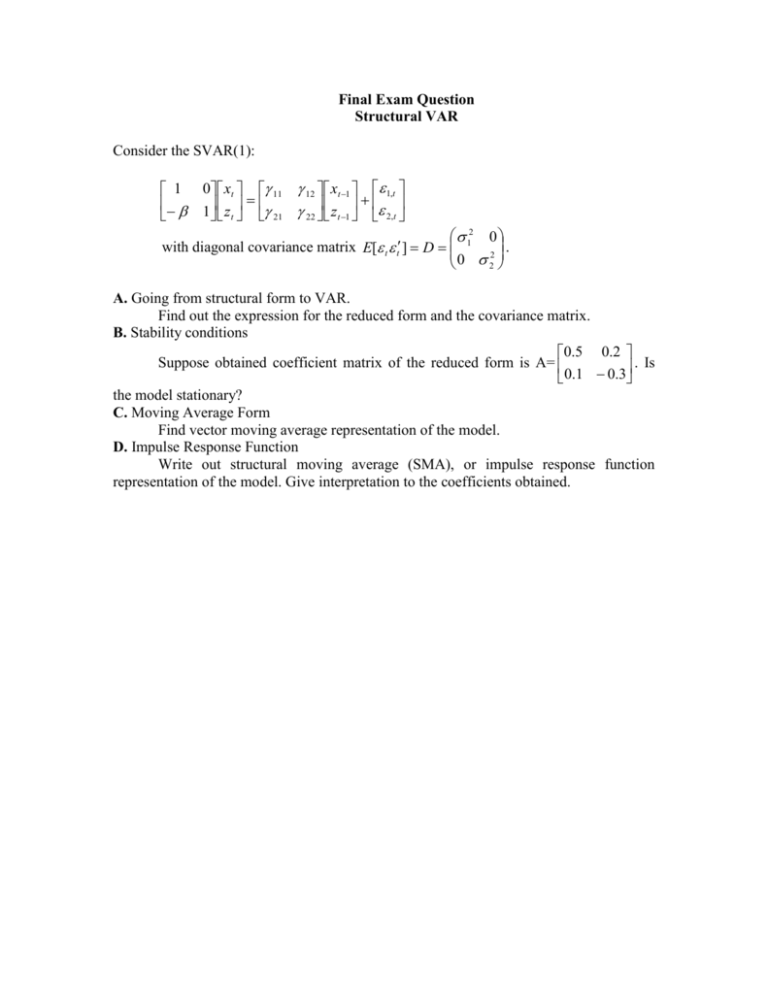
Final Exam Question
Structural VAR
Consider the SVAR(1):
 1
 

0  xt   11  12   xt 1   1,t 

 
1  z t   21  22   z t 1   2,t 
 12 0 
.
with diagonal covariance matrix E[ t  t ]  D  
2
0

2 

A. Going from structural form to VAR.
Find out the expression for the reduced form and the covariance matrix.
B. Stability conditions
0.5 0.2 
Suppose obtained coefficient matrix of the reduced form is A= 
 . Is
 0.1  0.3
the model stationary?
C. Moving Average Form
Find vector moving average representation of the model.
D. Impulse Response Function
Write out structural moving average (SMA), or impulse response function
representation of the model. Give interpretation to the coefficients obtained.
Key:
A. Going from structural form to VAR
VAR (the reduced form) is obtained by premultiplying by B 1 :
 1 0
1
B 1 
AdjB  1  

det B
  1
0  11  12   xt 1   1

1  21  22   z t 1   
A12   xt 1   u1,t 
 
A22   z t 1  u 2,t 
 xt   1
 z   
 t 
0  1,t    11
 
1  2,t    11   21

  xt 1    1,t





 12   22   z t 1   1,t   2,t 
 12
 A11
A
 21
As we see,  1,t  u1,t , so the first VAR shock equals the first structural shock. The second
VAR shock is a linear combination of the first two shocks. The covariance matrix of the
VAR shocks is therefore:
Var ( 1,t )
 u1,t 
   12
12 
1  Var ( 1,t )
1
1
Cov   B DB 



2
det 2 B  Var ( 1,t )  Var ( 1,t )  Var ( 2t )  12
 2 12   22 
u 2,t 
B. Stability conditions
The model is stationary when eigenvalues of A are all less than 1 in modulus.
0.2 
0.5  
det 
0
 0.3   
 0.1
(0.5   )( 0.3   )  0.02  0
 0.15  0.5  0.3  2  0.02  0
2  0.2  0.17  0
D  0.04  0.68  0.72
0.2  0.72
 0.32
2
0.2  0.72
2 
 0.52
2
So, this is a stable VAR.
1 
C. Moving Average Form
As we have no intercept, the VMA for our model is:
y t  u t  A1u t 1  A12 u t  2  ...
u
 u1,t 1 
 xt 
 u1t 
2  1,t  2 

I

A

A



  ...
2
1
1
z 
u 
 t
 2t 
u 2,t 1 
u 2,t 2 
 xt  1 0  u1t  0.5 0.2   u1,t 1  0.5 0.2  0.5 0.2   u1,t 2 
  ...
 z   0 1 u   0.1  0.3 u   0.1  0.3 0.1  0.3 u
  2t  
  2,t 1  

  2 ,t  2 
 t 
 xt   u1t  0.5 0.2   u1,t 1  0.27 0.04  u1,t 2 
  ...
 z   u   0.1  0.3 u   0.02 0.11 u
  2,t 1  
  2 ,t  2 
 t   2t  
D. Impulse Response Function
Substituting ut= B 1 εt into VMA gives SMA and thus impulse response function
representation of the model:
 xt   1 0  1t  0.5 0.2   1 0  1,t 1  0.27 0.04  1 0  1,t 2 
  ...
 z     1    0.1  0.3   1    0.02 0.11   1 
  2t  

  2,t 1  

  2 ,t  2 
 t 
 xt   1 0  1t  0.5  0.2  0.2   1,t 1  0.27  0.04  0.04  1,t 2 
  ...
 z     1     0.1  0.3  0.3     0.02  0.11 0.11 
  2t  
  2,t 1  
  2 ,t  2 
 t 
At time t+s :
 xt  s   1 0  1t  s  0.5  0.2  0.2   1,t  s 1  0.27  0.04  0.04  1,t  s 2 

  ...
 z     1     0.1  0.3  0.3 

  2t  s  
  2,t  s 1   0.02  0.11 0.11  2,t  s 2 
 t s  
Impulse response coefficients summarize how unit impulses of the structural
shocks at time t impact the level of dependent variables at time t + s for different values
of s. For example, for s=1 (0.5+02β) is the impulse response of x at time (t+1) to unit
change in ε1 at time t.