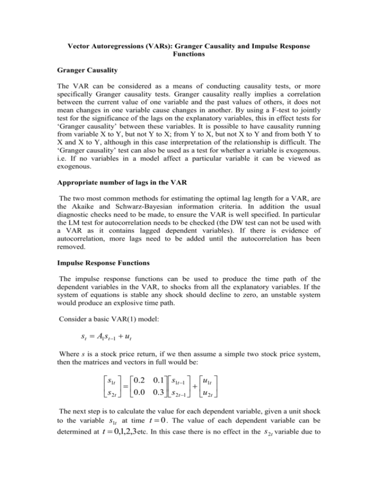
Vector Autoregressions (VARs): Granger Causality and Impulse Response
Functions
Granger Causality
The VAR can be considered as a means of conducting causality tests, or more
specifically Granger causality tests. Granger causality really implies a correlation
between the current value of one variable and the past values of others, it does not
mean changes in one variable cause changes in another. By using a F-test to jointly
test for the significance of the lags on the explanatory variables, this in effect tests for
‘Granger causality’ between these variables. It is possible to have causality running
from variable X to Y, but not Y to X; from Y to X, but not X to Y and from both Y to
X and X to Y, although in this case interpretation of the relationship is difficult. The
‘Granger causality’ test can also be used as a test for whether a variable is exogenous.
i.e. If no variables in a model affect a particular variable it can be viewed as
exogenous.
Appropriate number of lags in the VAR
The two most common methods for estimating the optimal lag length for a VAR, are
the Akaike and Schwarz-Bayesian information criteria. In addition the usual
diagnostic checks need to be made, to ensure the VAR is well specified. In particular
the LM test for autocorrelation needs to be checked (the DW test can not be used with
a VAR as it contains lagged dependent variables). If there is evidence of
autocorrelation, more lags need to be added until the autocorrelation has been
removed.
Impulse Response Functions
The impulse response functions can be used to produce the time path of the
dependent variables in the VAR, to shocks from all the explanatory variables. If the
system of equations is stable any shock should decline to zero, an unstable system
would produce an explosive time path.
Consider a basic VAR(1) model:
st  A1st 1  ut
Where s is a stock price return, if we then assume a simple two stock price system,
then the matrices and vectors in full would be:
 s1t  0.2 0.1  s1t 1  u1t 
 s   0.0 0.3  s   u 
  2t 1   2t 
 2t  
The next step is to calculate the value for each dependent variable, given a unit shock
to the variable s1t at time t  0 . The value of each dependent variable can be
determined at t  0,1,2,3etc. In this case there is no effect in the s 2 t variable due to
the way the model is set up, however if the s1t 1 variable had been significantly
different to zero, then the shock would have affected both variables.
s1  A1s0
u10 
Where s0  

u 20 
0.2 0.1 1  0.2
 0  0.0
0
.
0
0
.
3

   
This implies that: s1  
0.2 0.1 0.2 0.04
s2  A1s1  
   

0.0 0.3 0.0 0.0 
0.0008 
s3  A1s2  

0.0 
This process continue until the value of the dependent variable either becomes zero
(stable) or very large (unstable). We could have done the same process with s 2 t ,
although in this case the dependent variable would have been affected by both
explanatory variables, giving two separate time paths.
Variance Decomposition
This is an alternative method to the impulse response functions for examining the
effects of shocks to the dependent variables. This technique determines how much of
the forecast error variance for any variable in a system, is explained by innovations to
each explanatory variable, over a series of time horizons. Usually own series shocks
explain most of the error variance, although the shock will also affect other variables
in the system. It is also important to consider the ordering of the variables when
conducting these tests, as in practise the error terms of the equations in the VAR will
be correlated, so the result will be dependent on the order in which the equations are
estimated in the model.
Vector Error Correction Models
These are most associated with the VAR approach to cointegration, as before we can
form the VECM, we need to ensure the variables are cointegrated, as with the bivariate ECMs. There are other considerations though in this case, as if there is more
then one cointegrating vector, we can in theory have more than one error correction
term. However apart from this the VECM has the same properties as with the bivariate ECM.