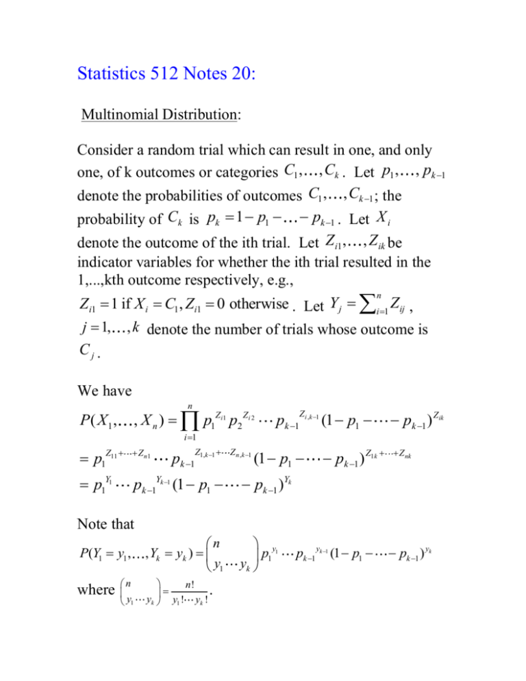
Statistics 512 Notes 20:
Multinomial Distribution:
Consider a random trial which can result in one, and only
one, of k outcomes or categories C1 , , Ck . Let p1 , , pk 1
denote the probabilities of outcomes C1 , , Ck 1 ; the
probability of Ck is pk  1  p1 
 pk 1 . Let X i
denote the outcome of the ith trial. Let Zi1 , , Zik be
indicator variables for whether the ith trial resulted in the
1,...,kth outcome respectively, e.g.,
n
Zi1  1 if X i  C1 , Zi1  0 otherwise . Let Yj  i 1 Zij ,
j  1,
Cj .
, k denote the number of trials whose outcome is
We have
n
, X n )   p1Zi1 p2 Zi 2
P( X 1 ,
i 1
Z1,k 1  Z n ,k 1
 p1Z11 
 Z n1
 p1Y1
pk 1Yk 1 (1  p1 
pk 1
pk 1
Zi ,k 1
(1  p1 
(1  p1 
 pk 1 ) Z1k 
 pk 1 ) Zik
 Z nk
 pk 1 )Yk
Note that
P(Y1  y1 ,
where
n

 y1
n
, Yk  yk )  
 y1

n!
.

yk  y1 ! yk !
 y1
p
yk  1
pk 1 yk 1 (1  p1 
 pk 1 ) yk
The likelihood is
l ( p1 ,
pk 1 )  Y1 log p1 
 Yk 1 log pk 1  (n  Y1 
Yk 1 ) log(1  p1 
 pk 1 )
The partial derivatives are:
Y n  Y1   Yk 1
l
 1 
p1 p1 1  p1   pk 1 ,...,
Y
n  Y1   Yk 1
l
 k 1 
pk 1 pk 1 1  p1   pk 1
Yj
It is easily seen that pˆ j , MLE  n satisfies these equations.
See (6.4.19) and (6.4.20) in book for information matrix.
Goodness of fit tests for multinomial experiments:
For a multinomial experiment, we often want to consider a
model with fewer parameters than p1 , , pk 1 , e.g.,
p1  f1 (1 , , q ), , pk 1  f k 1 (1 , ,  q ) (*)
where q  k  1 and ( , , )  
To test if the model is appropriate, we can do a “goodness
of fit” test which tests
H 0 : p1  f1 (1 , ,  q ), , pk 1  f k 1 (1 , ,  q ) for some (1 , ,  q )   vs.
H a : H 0 is not true for any (1 , , q )
1
q
We can do this test using a likelihood ratio test where the
number of extra parameters in the full parameter space is
D
(k  1)  q
2
so that 2 log    (( k  1)  q) under H 0 .
Example 2: Linkage in genetics
Corn can be starchy (S) or sugary (s) and can have a green
base leaf (G) or a white base leaf (g). The traits starchy and
green base leaf are dominant traits. Suppose the alleles for
these two factors occur on separate chromosomes and are
hence independent. Then each parent with alleles SsGg
produces with equal likelihood gametes of the form (S,G),
(S,g), (s,G) and (s,g). If two such hybrid parents are
crossed, the phenotypes of the offspring will occur in the
proportions suggested by the able below. That is, the
probability of an offspring of type (S,G) is 9/16; type (SG)
is 3/16; type (S,g) 3/16; type (s,g) 1/16.
Alleles of first parent
Alleles
SG
Sg
of
SG
(S,G) (S,G)
second Sg
(S,G) (S,g)
parent sG
(S,G) (S,G)
Sg
(S,G) (S,g)
sG
(S,G)
(S,G)
(s,G)
(s,G)
sg
(S,G)
(s,G)
(s,G)
(s,g)
The table below shows the results of a set of 3839 SsGg x
SsGg crossings (Carver, 1927, Genetics, “A Genetic Study
of Certain Chlorophyll Deficiencies in Maize.”)
Phenotype
Starchy green
Starchy white
Sugary green
Sugary white
Number in sample
1997
906
904
32
Does the genetic model with 9:3:3:1 ratios fit the data?
Let X i denote the phenotype of the ith crossing.
Model: X 1 , , X n are iid multinomial.
P( X i  SG )  pSG , P( X i  Sg )  pSg , P( X i  sG )  psG , P( X i  sg )  psg
H 0 : pSG  9 /16, pSg  3/16, psG  3/16, psg  1/16
H1 : At least one of pSG  9 /16, pSg  3/16, psG  3/16, psg  1/16 is not correct.
Likelihood ratio test:
max  L( )
(9 /16)1997 (3 /16)906 (3 /16)904 (1/16)32


max  L( ) (1997 / 3839)1997 (906 / 3839)906 (904 / 3839)904 (32 / 3839)32
9 /16
3 /16
 906 log

1997 / 3839
906 / 3839
3/16
1/16
904log
 32 log
)  387.51
904/3839
3839
2 log   2*(1997 log
Under H 0 : pSG  9 /16, pSg  3 /16, psG  3 /16, psg  1/16 ,
2 log  ~  2 (3) [there are three extra free parameters in
H1 ].
2
Reject H 0 if 2 log   .05 (3)  7.81 .
Thus we reject
H 0 : pSG  9 /16, pSg  3 /16, psG  3 /16, psg  1/16 .
Model for linkage:
1
1
1
1
pSG  (2   ), pSg  (1   ), psG  (1   ), psg  
4
4
4
4
Y
Y
Y
1
2
3
1
 1
 1
 1 
L( )   (2   )   (1   )   (1   )    
4
 4
 4
 4 
n Y1 Y2 Y3
Maximum likelihood estimate of  for corn data = 0.0357,
see handout.
Test
1
1
1
1
(2   ), pSg  (1   ), psG  (1   ), psg   vs.
4
4
4
4
H1 : pSG , pSg , psG , psg do not satisfy
H 0 : pSG 
1
1
1
1
(2   ), pSg  (1   ), psG  (1   ), psg  
4
4
4
4
for any  ,0    1
pSG 

max  L( ) (.25*(2  .0357))1997 (.25*(1  .0357))906 (.25*(1  .0357))904 (.25*.0357)32

max  L( )
(1997 / 3839)1997 (906 / 3839)906 (904 / 3839) 904 (32 / 3839)32
2 log   2.02
2
Under H 0 , 2 log  ~  (2) [there are two extra free
parameters in H1 ].
2
2 log   .05
(2)  5.99
Linkage model is not rejected.
Sufficiency
Let X 1 , , X n denote the a random sample of size n from a
distribution that has pdf or pmf f ( x; ) . The concept of
sufficiency arises as an attempt to answer the following
question: Is there a statistic, a function
Y  u ( X1 , , X n ) which contains all the information in the
sample about  . If so, a reduction of the original data to
this statistic without loss of information is possible. For
example, consider a sequence of independent Bernoulli
trials with unknown probability of success  . We may
have the intuitive feeling that the total number of successes
contains all the information about  that there is in the
sample, that the order in which the successes occurred, for
example, does not give any additional information. The
following definition formalizes this idea:
Definition: Let X 1 , , X n denote the a random sample of
size n from a distribution that has pdf or pmf f ( x; ) ,
  . A statistic Y  u ( X1 , , X n ) is said to be sufficient
for  if the conditional distribution of X 1 , , X n given
Y  y does not depend on  for any value of y .
Example 1: Let X 1 ,
, X n be a sequence of independent
Bernoulli random variables with P( X i  1)   . We will
verify that Y  i 1 X i is sufficient for  .
Consider
P ( X1  x1 , , X n  xn | Y  y)
n
For y  i 1 xi , the conditional probability is 0 and does
not depend on  .
n
For y  i 1 xi ,
n
P ( X 1  x1 ,
, X n  xn | Y  y ) 
P ( X 1  x1 , , X n  xn , Y  y )
P (Y  y )
 y (1   )n  y
1


n  y
n
n y
   (1   )
 
 y
 y
The conditional distribution thus does not involve  at all
and thus Y  i 1 X i is sufficient for  .
n
Example 2:
Let X 1 , , X n be iid Uniform( 0,  ). Consider the statistic
Y  max1i n X i .
We have shown before (see Notes 1) that
 ny n 1
0  y 

fY ( y )    n
0
elsewhere

For Y   , we have
P ( X 1  x1 ,
, X n  xn | Y  y ) 
P ( X 1  x1 , , X n  xn | Y  y )
P (Y  y )
1
I
n Y 
1

 n 1
 n 1
ny
n
IY 
ny
which does not depend on  .
For Y   , P ( X1  x1 , , X n  xn | Y  y)  0 .
Thus, the conditional distribution does not depend on 
and Y  max1i n X i is a sufficient statistic
Factorization Theorem: Let X 1 , , X n denote the a random
sample of size n from a distribution that has pdf or pmf
f ( x; ) ,   . A statistic Y  u ( X1 , , X n ) is sufficient
for  if and only if we can find two nonnegative functions,
k1 and k2 such that
f ( x1; ) f ( xn ; )  k1[u( x1 , , xn ); ]k2[( x1 , , xn )]
where k2 [( x1 ,
, xn )] does not depend upon  .