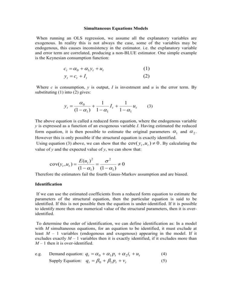
Simultaneous Equations Models
When running an OLS regression, we assume all the explanatory variables are
exogenous. In reality this is not always the case, some of the variables may be
endogenous, this causes inconsistency in the estimator. i.e. the explanatory variable
and error term are correlated, producing a non-BLUE estimator. One simple example
is the Keynesian consumption function:
ct   0  1 yt  ut
(1)
yt  ct  I t
(2)
Where c is consumption, y is output, I is investment and u is the error term. By
substituting (1) into (2) gives:
yt 
0
1
1

It 
ut
(1  1 ) 1  1
1  1
(3)
The above equation is called a reduced form equation, where the endogenous variable
y is expressed as a function of an exogenous variable I. Having estimated the reduced
form equation, it is then possible to estimate the original parameters 1 and  2 .
However this is only possible if the structural equation is exactly identified.
Using equation (3) above, we can show that the cov( yt , ut )  0 . By calculating the
value of y and the expected value of y, we can show that:
cov( yt , ut ) 
E (ut ) 2
2

0
(1  1 ) (1  1 )
Therefore the estimators fail the fourth Gauss-Markov assumption and are biased.
Identification
If we can use the estimated coefficients from a reduced form equation to estimate the
parameters of the structural equation, then the particular equation is said to be
identified. If this is not possible then the equation is under-identified. If it is possible
to identify more then one numerical value of the structural parameters, then it is overidentified.
To determine the order of identification, we can define identification as: In a model
with M simultaneous equations, for an equation to be identified, it must exclude at
least M – 1 variables (endogenous and exogenous) appearing in the model. If it
excludes exactly M – 1 variables then it is exactly identified, if it excludes more than
M – 1 then it is over-identified.
e.g.
Demand equation: qt   0  1 pt   2it  ut
Supply Equation: qt   0  1 pt  vt
(4)
(5)
Where we assume I is exogenous and p and q are endogenous. The first equation is
not identified (2-1=1), there are no variables excluded from this equation. The second
equation is just identified (2-1=1), there is exactly one variable (I) excluded.
Vector Autoregression (VAR)
The VAR is often perceived as an alternative to the simultaneous equation method. It
is a systems regression model in that there is more than one dependent variable. In the
most basic bivariate example, where there are just two variables, then each of their
current values will depend on combinations of the previous values of both variables
and error terms.
yt   0   1 xt 1   1 yt 1 .....   k xt k   k yt k  u t
xt   0   1 xt 1   1 yt 1 ......   k xt k   k yt k  vt
The number of lags included in the VAR depends on either the data (i.e. monthly data
would require 12 lags) or minimizing the Akaike or Schwarz-Bayesian criteria (
maximising in some text books depending on how the criteria is set up). In addition it
is assumed that the error term is not serially correlated. The system can be expanded
to include any number of variables and is used extensively in the Finance literature.
The VAR has various advantages over univariate time series models, for instance
there is no need to specify which variables are exogenous and which endogenous, all
variables are by definition endogenous. (However it is possible to specify a purely
exogenous variable as a regressor, in this case there would be no equation in which it
was a dependent variable). In addition the problem of model identification does not
occur when using a VAR. Providing there are no contemporaneous terms acting as
regressors, OLS can be used to estimate each equation individually, as all the
regressors are lagged so therefore treated as pre-determined. In addition VARs are
often highly efficient at forecasting compared to traditional models.
However the VAR approach has some very important defects, it is viewed as atheoretical. As the model specification tends not to be driven by theory. It is also
difficult to know the appropriate lag lengths to include in the VAR, different methods
often suggest different numbers of lags. If large numbers of lags are included, many
will often be insignificant and if there are a large number of equations in the VAR
then a large number of degrees of freedom would be required. It is also difficult to
interpret the coefficients and levels of significance, the lags are often tested for joint
significance. In addition the number of lags for each equation will be the same, unless
specific restrictions are applied to each equation. Finally should each component of
the VAR be treated as stationary, first-differencing results in a loss of long-run
information. A way around this problem is to use a Vector Error Correction Model
(VECM).