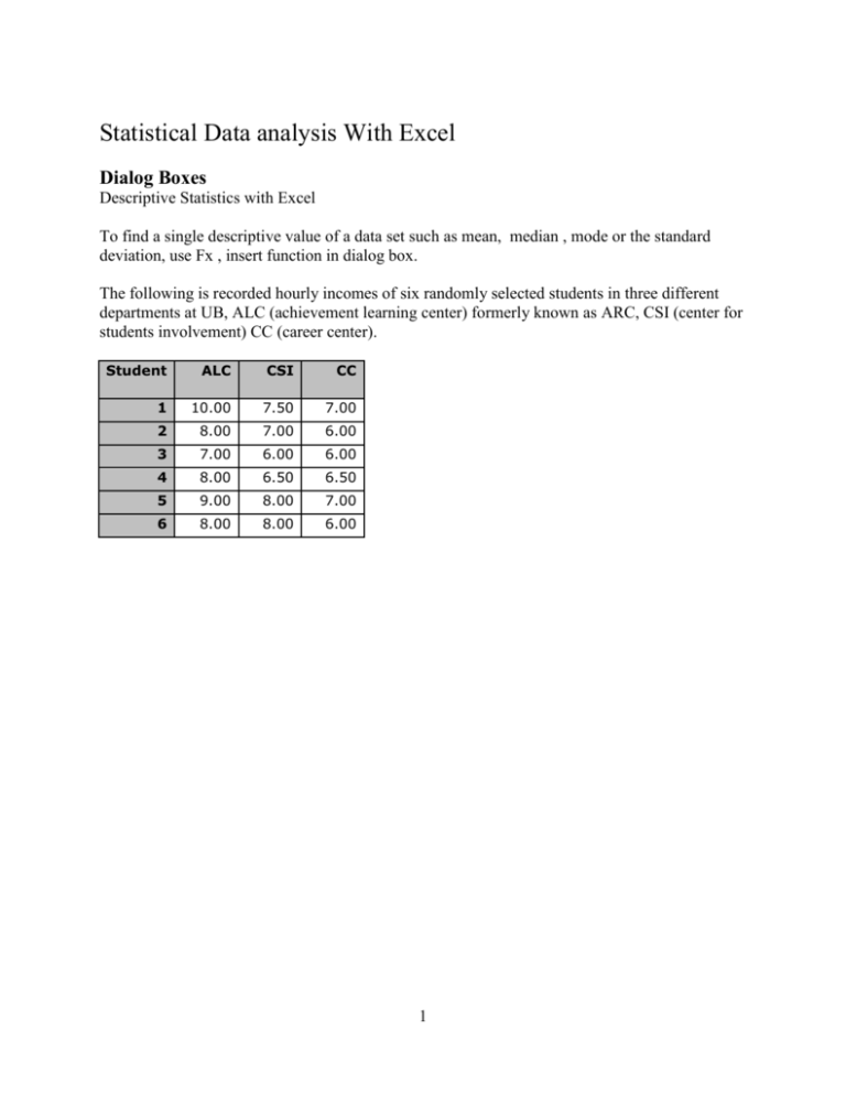
Statistical Data analysis With Excel
Dialog Boxes
Descriptive Statistics with Excel
To find a single descriptive value of a data set such as mean, median , mode or the standard
deviation, use Fx , insert function in dialog box.
The following is recorded hourly incomes of six randomly selected students in three different
departments at UB, ALC (achievement learning center) formerly known as ARC, CSI (center for
students involvement) CC (career center).
Student
ALC
CSI
CC
1
10.00
7.50
7.00
2
8.00
7.00
6.00
3
7.00
6.00
6.00
4
8.00
6.50
6.50
5
9.00
8.00
7.00
6
8.00
8.00
6.00
1
2
3
Imagine you want to find mean, median , mode of hourly incomes of only students who are
working for the ALC.
The result will be placed on the designated cell where the Fx is activated.
4
To find the mean of CSI and CC students, you can copy F8 and paste on G8 and H8.
Similarly you can find other quantities for each column for a particular range of data but you
have to get yourself familiar with abbreviation for these quantities from the insert function.
Examples of these abbreviations are:
Average  mean
Var
 Variance
Median  Median
Mode  Mode
Max
 Maximum
STDEV  Standard deviation
We can also use a single operation to find these quantities altogether in one step. To do so before
entering any data into Excel spread sheet, make sure to install data Analysis Tool Pack on your
Excel.
5
The following steps can be taken to load Excel’s Analysis Toolpak from addin dialog :
The Analysis ToolPak is a Microsoft Office Excel add-in program that is available when you install Microsoft Office or
Excel. To use it in Excel, however, you need to load it first.
1.Click the Microsoft Office Button
, and then click Excel Options.
2. Click Add-Ins, and then in the Manage box, select Excel Add-ins.
3. Click Go.
4.In the Add-Ins available box, select the Analysis ToolPak check box, and then click OK. Tip If Analysis
ToolPak is not listed in the Add-Ins available box, click Browse to locate it.If you get prompted that the Analysis
ToolPak is not currently installed on your computer, click Yes to install it.
5.After you load the Analysis ToolPak, the Data Analysis command is available in the Analysis group on
the Data tab.
Now imagine you want to find several descriptive factors of a variable using a function not
several at a time.
To show you some basic Statistical Data Analysis, I recorded hourly incomes of six students in
three different departments at UB.
Student
ALC
CSI
CC
1
2
3
4
5
6
10.00
8.00
7.00
8.00
9.00
8.00
7.50
7.00
6.00
6.50
8.00
8.00
7.00
6.00
6.00
6.50
7.00
6.00
To find all descriptive statistics values of a set of data such as ARC students hourly income, from
the menus:
Choose
Tools
Data Analysis
Descriptive Statistics
Ok
Then enter range of data and click on Label Included if the range
includes the Label, enter the range of you output, for exampleB9 also
click on summary statistics then OK.
In the output range, the following will be displayed
6
In descriptive statistics dialog we also check on confidence interval for mean in order to be able
to find a 95% confidence interval for the mean of the population this sample is taken from.
7
8
Based on sample information we can be 95% confident that the true mean of population is
between 8.33333333 - 1.08385247 and 8.33333333 + 1.08385247 or from 7.24948086 to
10.4171858. The confidence level in this output represents margin of error.
9
Normal distribution
A distribution is normal if the three measures of locations mean, median and mode are equal. We
also assume a distribution is normal if these three measures are roughly equal. General shape of a
normal distribution looks like a bell curved figure. The mean of distribution is located in the
middle. Fifty percent of all observations are in the left and the other fifty percent are in the right
side of the mean. Before we use a standard table to find certain probabilities an observation in a
normal distribution, we should learn a rule of thumb for certain percentage in a normal
distribution. These rules are called empirical rules:
1) In a normal distribution approximately 68% of all observations are within one standard
deviation from the mean. Graphical elastration of this fact look like:
For example we know IQ scores are normal with mean of 100 and standard deviation 10. Based
on empirical rule number one we can say approximately middle 68% of all IQ scores are within:
100 – 10 and 100 + 10 or within 90 and 110.
10
2) Similarly we can say, in a normal distribution approximately 95% of all observations
are within two standard deviations from the mean. Graphical elastration of this fact look
like:
For example we know IQ scores are normal with mean of 100 and standard deviation 10. Based
on empirical rule number two we can say approximately middle 95% of all IQ scores are within:
100 – 2X10 and 100 + 2X10 or within 80 and 120.
11
3) Virtually all or 99.7% of all observations are within three standard deviations from the
mean. Graphically looks like:
In this case, we know also use IQ scores that are normal with mean of 100 and standard
deviation 10. Based on empirical rule number three we can say approximately middle 99.7% of
all IQ scores are within 100 – 3X10 and 100 + 3X10 or within 70 and 130.
12
Now let’s use Excel to find the probability of getting less than a value from a normal curve.
Normal Distribution Functions in Excel
A distribution is normal if the mean , median and the mode in that distribution are equal or
roughly equal. The general shape of a normal distribution is bell shaped with mean in the middle
where 50% of all observations are in the left and the other 50% of all observations are in the
right side of the mean. We could use direct and indirect functions NORMDIS , NORMINV or
NORMSINV to find probability of getting observations below a certain observation or the
corresponding Percentile of an observation. To have a better understating of problems dealing
with normal curve lets solve the following problem.
Problem
Assume mathematics part of the GRE examination is normal with mean of µ=500 and the
standard deviation of σ =100. Answer the following questions:
1) What is the probability that a randomly selected test taker scores less than 650 points?Or
we can say what is the percentile rank of a person with score 650 points.
Solution: If you wish to solve this problem by hand it would be appropriate to
have a normal distribution table and always to draw a bell shaped
graph to have a clear understanding of the question. We locate the
given observation in this case x =650 in right hand side of the mean
µ=500 and calculate its norm Z-score. The area to the left side of the Z
score of 650(Z= 1.5) is the answer. The answer from a normal curve
is 0.9332 or approximately 93.32%.
If you want to find the probability by Excel, from Fx functions, use NORMDIS as
followed. The percentile rank of this person is 93.32%.
13
14
Simple Regression and correlation procedure
In simple regression study we would to see whether there is a relationship between two
variables, the dependent and the independent variable. As you recall from basic algebra class
we used letter y for dependent and the letter x for independent variable. If the relationship
between the two variables is proven to be linear then we can predict the value of dependent
variable based on value of independent variable. The basic formula from algebra class is y =
mx + b. In this formula m is the slope of the line and b is the y-intercept of the line. Real life
example could be an example like y = 2 x + 10 assuming y is the dollar value of a stock and x
is the age of the stock in years. In this formula +2 is the yearly increase and 10 is the value of
stock at inception that is year zero or year x = 0. If this is a fit model then we can say this
stock is worth y = 2(10) + 10 = 30 or $30 ten years from now. It is very important to be able to
explain the slope and the y-intercept in conjunction with the problem statement. To make
this clear lets use a simple problem in a real life situation.
Example: As a college administer, I am interested to see whether there is a
relationship between hourly rate of students working for CC (y) and
students working for the ALC(x). Also I would like to be able to predict hourly
income of a student working for CC based on his or her hourly rate when
he or she was working for the ALC.
15
ALC=ARC(x), TCC=CC(y)
Student
ALC(x)
CSI
CC(y)
1
10.00
7.50
7.00
2
8.00
7.00
6.00
3
7.00
6.00
6.00
4
8.00
6.50
6.50
5
9.00
8.00
7.00
6
8.00
8.00
6.00
From Analysis Tool, select Regression then enter the range of data as specified.
The output clearly contains a lot of values which calculation of those values by
hand using appropriate formulas is very time consuming. The following screen
shots provide you a clear approach in solving this and problems similar to it.
Notice we only have six pair points to deal with in this case but the procedure
can be used for as many as 65000 pair points entered in an Excel spread sheet.
16
17
18
Referring to this output, first we investigate whether the correlation between the two variables
is strong. To do so we refer to the P-value of the slope of the line that is 0.0306246 taken from
the output. Because this P-value is less than 0.05, we reject the null hypothesis. The null
hypothesis in this case indicate that slope is equal to zero (no correlation) and the alternative
indicates that slope is not equal to zero(strong correlation).
Since we found a strong correlation between the two variables we can write an equation that
predicts one variable(y) given the other variable (x). The model in this case is:
Y = 0.40625X + 3.03125 or
TCC hourly rate = 0.40625(ARC hourly rate) + 3.03125.
Imagine a student was working for the ALC at hourly rate of $10 and quit and went on to work
for CC, what would be the hourly income of this student at TCC?
TCC = 0.40625(10) + 3.03125 = $7.09 this is the predicted hourly income of the student at CC.
From the original table the actual value of y when x was $10 is $7 this gives a residual of 7 –
7.09=-0.09 that indicates a good prediction. Residual analysis in regression studies are very
important but very time consuming to explain. Of course, you will possibly be asked to do so in
your PUAD 628 class.
19
Multiple Regressions
You can similarly find a model when you have one dependent variable and several independent
variables. The model will look like:
y= b0 +m1x1+ m2x1+…. You will see several slopes but the same y-intercept. Imagine you want
to estimate the percentage chance of a person stroke based on his or her age, blood pressure and
whether or not the person smokes. In this case we convert the nominal scale of smoking from
yes to 1 and from no to 0. To see a better picture of a problem such as this one lets refer to a
problem statement and answer a some questions after completion of multiple regression data
analysis.
Problem statement
The American Heart Association collects data on the risk of strokes. A 10-year study provided
data on how age, blood pressure, and smoking related to the risk of strokes (U.S. News & World
Report, April 13, 1992). Assume that following data are from a portion of this study. Risk is
interpreted as the probability (times 100 ) that the patient will have a stroke over the next 10-year
period. For the smoking variable, define a dummy variable with 1 indicating a smoker and 0
indicting a non-smoker.
RISK%
AGE
BLOOD SMOKER
PRESSURE
12
57
152
0
24
67
163
0
13
58
155
0
56
86
177
1
28
59
196
0
51
76
189
1
18
56
155
1
31
78
120
0
37
80
135
1
15
78
98
0
22
71
152
0
36
70
173
1
15
67
135
1
48
77
209
1
15
60
199
0
36
82
119
1
8
66
166
0
34
80
125
1
3
62
117
0
37
59
207
1
20
21
22
SUMMARY OUTPUT
Regression Statistics
Multiple R
0.93461
R Square
0.87349
Adjusted R
Square
0.84977
Standard Error
5.75657
Observations
20
ANOVA
df
Regression
Residual
Total
3
16
19
Coefficients
Intercept
AGE
BLOOD
PRESSURE
SMOKER
-91.7595
1.07674
0.25181
8.73987
SS
MS
F
3660.739588 1220.25 36.82301
530.2104116 33.1382
4190.95
Standard Error
t Stat
15.22276009 6.02778
0.165963611 6.48781
P-value
Significance
F
2.06404E-07
Lower 95%
Upper 95%
Lower 95.0%
1.76E-05 -124.030308 -59.488689 -124.030308
7.49E-06 0.724913921 1.42856819 0.724913921
0.045225519 5.56795 4.24E-05 0.155939657 0.34768729 0.155939657
3.000815432 2.9125 0.010174 2.378426561 15.1013155 2.378426561
As you see there is a strong correlation between the chance of stroke and all of the other variables. The pvalue of age is 7.49E-06 =0.00000749, the p-value of blood pressure is 4.24E-05 =0.0000424 and the pvalue of smoking is 0.010174. All of these p-values are less than 0.05 hence the correlation between the
chance of stroke and all of the other variables is strong positive correlation. The estimated regression
line is:
Y = -91.7595 + 1.07674 X1 + 0.25181 X2 + 8.73987 X3 or
% chance of stroke = -91.7595 + 1.07674 (age) + 0.25181 (blood pressure) +8.739879(smoking)
We should be able to explain each slope in conjunction with the problem statement and also be able to
predict the chance of stroke for a person if we are given age, blood pressure and know whether the
person smokes or not. Let me calculate my risk of stroke at my age of 57 years, blood pressure of 125
and knowing that I don’t smoke.
% risk of stroke = = -91.7595 + 1.07674 (57) + 0.25181 (125) +8.739879(0)=1.09%
23