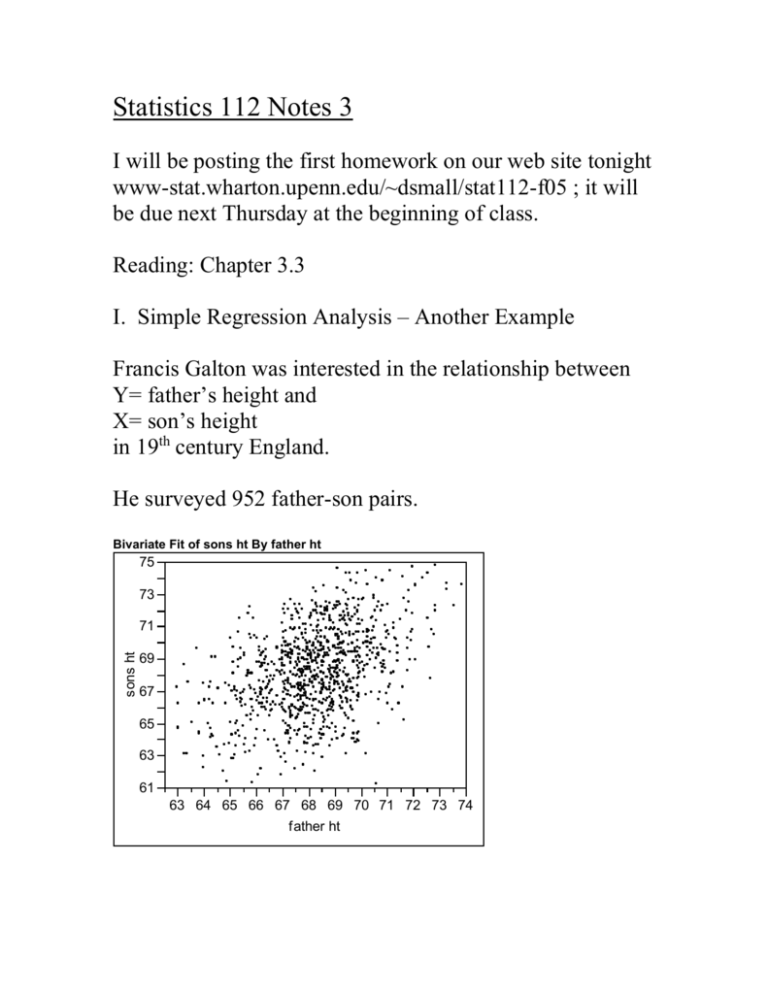
Statistics 112 Notes 3
I will be posting the first homework on our web site tonight
www-stat.wharton.upenn.edu/~dsmall/stat112-f05 ; it will
be due next Thursday at the beginning of class.
Reading: Chapter 3.3
I. Simple Regression Analysis – Another Example
Francis Galton was interested in the relationship between
Y= father’s height and
X= son’s height
in 19th century England.
He surveyed 952 father-son pairs.
Bivariate Fit of sons ht By father ht
75
73
sons ht
71
69
67
65
63
61
63 64 65 66 67 68 69 70 71 72 73 74
father ht
Simple regression analysis seeks to estimate the mean of
son’s height given father’s height, E(Y|x).
The simple linear regression model is
E (Y | x)  0  1 x
To estimate 0 , 1 , we use the least squares method.
Using our sample of data, we estimate 0 , 1 by
b0 , b1 where b0 , b1 are chosen to minimize the sum of
squared prediction errors in the data (the least squares
method).
Bivariate Fit of sons ht By father ht
75
73
sons ht
71
69
67
65
63
61
63 64 65 66 67 68 69 70 71 72 73 74
father ht
Linear Fit
Linear Fit
sons ht = 26.455559 + 0.6115222 father ht
Each one inch increase in father’s height is (estimated to
be) associated with an increase in mean son’s height of
0.61 inches.
II. Simple Linear Regression Model Assumptions
The sample data (Y1 , X1 ),
population.
, (Yn , X n ) is a sample from a
We care about learning about the mean of Y given X in the
population not in the sample, e.g.,
 The real estate agent from Lecture 2 who did the
regression of X=house size on Y=selling price was
interested in the relationship between these variables
for all houses in Gainesville, FL not just the 93 houses
in her sample.
 Galton is interested in how father’s height relates to
son’s height in all of England, not just among these
952 father-son pairs.
The least squares method provides estimates b0 , b1 of
0 , 1 based on the sample – these estimates will differ for
differ samples and typically will not exactly be correct.
Standard errors and confidence intervals for 0 , 1 are used
to quantify our uncertainty about 0 , 1 .
To compute standard errors and confidence intervals, we
need to have a model for how the data arises from the
population.
The simple linear regression model:
Yi  0  1 xi  ei .
The ei are called disturbances and it is assumed that
1. Linearity assumption: The conditional expected value
of the disturbances given xi is zero, E (ei )  0 , for
each i. This implies that E (Y | x)  0  1 x so that the
expected value of Y given X is a linear function of X.
2. Constant variance: assumption: The disturbances
ei are assumed to all have the same variance  2 .
3. Normality assumption: The disturbances ei are
assumed to have a normal distribution.
4. Independence assumption: The disturbances ei are
assumed to be independent. This is an assumption that
is most important when the data are gathered over
time. When the data are cross-sectional (that is,
gathered at the same point in time for different
individual units), this is typically not an assumption of
concern.
Steps in simple regression analysis:
1. Observe pairs of data (x1,y1),…,(xn,yn) that are a
sample from population of interest.
2. Plot the data.
3. Assume simple linear regression model assumptions
hold.
4. Estimate the true regression line
E (Y | x)  0  1 x by the least squares line
Eˆ (Y | x)  b  b x .
0
1
5. Check whether the assumptions of the ideal model are
reasonable (Chapter 6). If assumptions don’t hold,
consider transforming some of the variables (Chapter
5).
6. Make inferences concerning coefficients 0 , 1
and make predictions ( ŷ  b0  b1 x ).