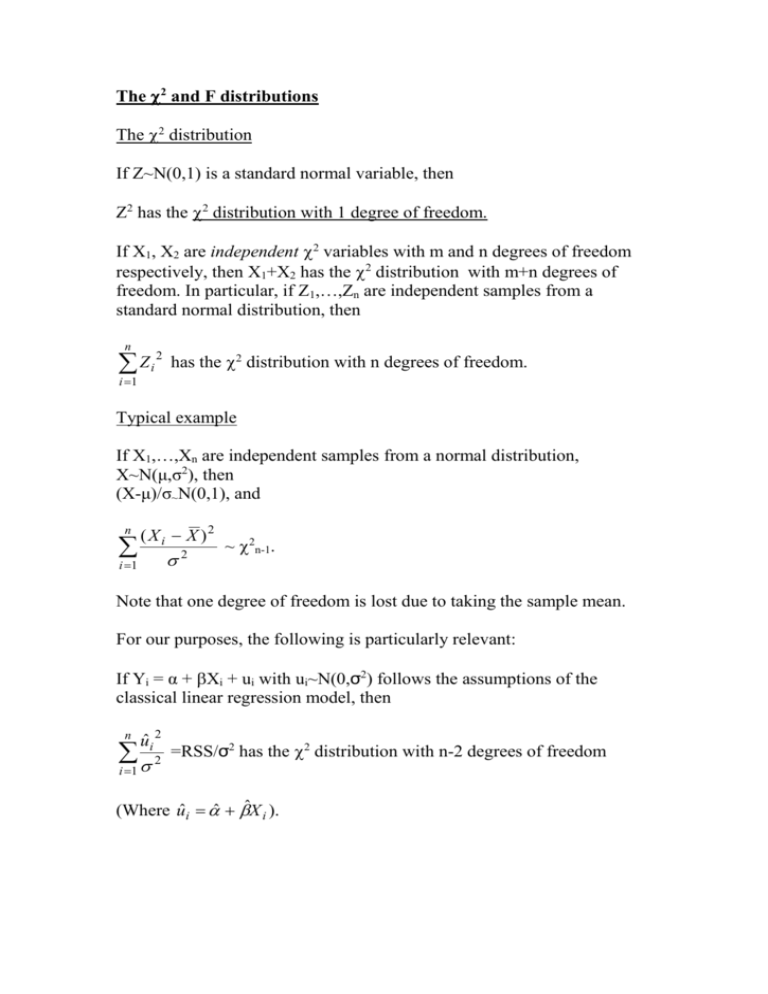
The 2 and F distributions
The 2 distribution
If Z~N(0,1) is a standard normal variable, then
Z2 has the 2 distribution with 1 degree of freedom.
If X1, X2 are independent 2 variables with m and n degrees of freedom
respectively, then X1+X2 has the 2 distribution with m+n degrees of
freedom. In particular, if Z1,…,Zn are independent samples from a
standard normal distribution, then
n
 Zi 2
has the 2 distribution with n degrees of freedom.
i 1
Typical example
If X1,…,Xn are independent samples from a normal distribution,
X~N(μ,σ2), then
(X-μ)/σ~N(0,1), and
n

( X i  X )2

i 1
2
~ 2n-1.
Note that one degree of freedom is lost due to taking the sample mean.
For our purposes, the following is particularly relevant:
If Yi = α + Xi + ui with ui~N(0,σ2) follows the assumptions of the
classical linear regression model, then
n
uˆi 2
 2
=RSS/σ2 has the 2 distribution with n-2 degrees of freedom
i 1
(Where uˆi  ˆ  ˆX i ).
In general, if we have k explanatory variables, X1,…,Xk in our regression
n
uˆi 2
model, then  2 ~ 2n-k-1.
i 1 
Relationship between the t-statistic and the 2 statistic
The t-distribution is initially defined in terms of the standard normal and
the 2 distribution.
Let Z~N(0,1), and let X~2n , with the two variables independent.
Then
Z
has the t-distribution with n degrees of freedom.
X /n
Example: Let X1,…,Xn be independent samples from a normal
distribution, Xi~N(μ,σ2).
Then
(X  )
~N(0,1)
( / n )
n
While

( X i  X )2

i 1
2
~ 2n-1.
It can be shown that these two variables are independent. Hence,
(X  )
( / n )

n
 ( X i  X ) 2 /(n  1)
i 1

(X  )
n
 ( X i  X ) 2 /(n  1)
n
i 1
(X  ) (X  )
=
~ tn-1, which is exactly how we introduced the tˆ 2 / n S .E.( X )
distribution in the first place.
=
For regression purposes, we know that the regression coefficient
2
ˆ
ˆ
ˆ
 ~N(,Var(  )), where Var(  )= n
 ( X i  X )2
i 1
Hence
( ˆ   )

~ N(0,1).
2
 ( X i  X )2
n
uˆi 2
 2
We also have that
~ 2n-2 , and it can be shown that these two
i 1
variables are independent.
Dividing the standard normal variable by the root of the 2 variable over
its degrees of freedom, and cancelling the sigma, we get
( ˆ   )
( uˆi 2 ) /( n  2)
 ( X i  X )2

( ˆ   )
ˆ 2 /  ( X i  X ) 2
=
( ˆ   )
S .E.( ˆ )
Has the t-distribution with n-2 degrees of freedom. A similar result holds
for the k-variable case.
The F-distribution
Let X1 and X2 be independent 2 variables with n1 and n2 degrees of
freedom respectively. Then (X1/n1)/(X2/n2) has the F-distribution with
(n1,n2) degrees of freedom.
The F-distribution can be used for comparing the variances of two normal
distributions. In regression analysis, it is absolutely crucial, for testing
restrictions on the regression model, and in particular, testing the
restriction that all the explanatory variables are insignificant.
n
2
We have already seen that the RSS/σ ,
uˆi 2
 2
i 1
~ 2n-k-1.
It can be shown that, in the classical regression model, the Explained Sum
(Yˆi  Y ) 2

2
of Squares (ESS) divided by σ , that is
has the 2
2

distribution with k degrees of freedom, under the assumption of the null
hypothesis, that all the explanatory variables are insignificant, that is that
the true values of 1,…,k are zero.
Hence, dividing and cancelling the σ2, we get that, under the null
hypothesis
F
ESS / k
~F(k,n-k-1)
RSS /( n  k  1)
We may therefore compare the resulting F statistic with the 95% or 99%
etc. critical value of the appropriate F distribution. If the F-statistic
exceeds this critical value, we may reject the null hypothesis that
1=2=….=k=0, and conclude that the regression as a whole is
significant, that is that the variables X1,…,Xk are jointly significant.
It is possible for a set of variables to be jointly significant, even if they
are all individually insignificant. This is particularly likely if there is a
very close relationship between the X-variables (multicolinearity); it may
be possible to tell that the variables together are insignificant, but
impossible to separate out the effect of just one of them, because they are
so closely linked. E.g. consider the effect of income and wealth on
consumption – income and wealth are very strongly correlated, so while
they would certainly be jointly significant, it may be impossible to
separate out their effects.
More generally, suppose we have a model with a number of X variables,
and we wish to test the hypothesis that some of them are jointly
insignificant. That is, suppose we estimate the model
Yi = α+1X1i+…+kXki + ui , and we wish to test the hypothesis that
1 = … = l =0, with l≤k – that is, we are testing the hypothesis that
X1,…,Xl are jointly insignificant. It can be shown that the difference
between the RSS obtained with the original model, and the RSS obtained
with the restricted model (with the first l variables removed), divided by
σ2, has the 2 distribution with l degrees of freedom, under the null
hypothesis that 1 = … = l =0.
Let RSS1 be the RSS obtained with the unrestricted model, and let RSS2
be the RSS from the restricted model, that is with 1=…=l=0. Then
under the null hypothesis,
F=
( RSS2  RSS1 ) / l
~ F(l,n-k-1).
RSS1 /( n  k  1)
(Note that RSS2 will be greater than RSS1 – since we have fewer
variables in the restricted model, the residuals will be higher.)
We may therefore compare this F statistic with the appropriate critical
value of the F distribution. If the statistic exceeds the 95% (or 99% or
whatever) critical value, then we may reject the null hypothesis, and
conclude that the deleted variables, X1,…,Xl, are in fact significant.
More generally still, the same statistic can be used when testing any l
linear restrictions on the model – for example, a linear restriction may
take the form 1=1, or 1+2=0, etc. Here, RSS2 is the RSS from the
regression obtained by imposing these restrictions, that is by calculating
the least squares estimators based on the requirement that these are true.
For example, suppose our model is
Yi = α+1X1i+2X2i+3X3i + ui, and we are testing the hypothesis that
1=1 and 2+3=0, then the restricted model involves finding estimators
for the model
Yi=α + X1i + 2X2i - 2X3i + ui. Hence we choose α and 2 to minimise the
sum of square error.