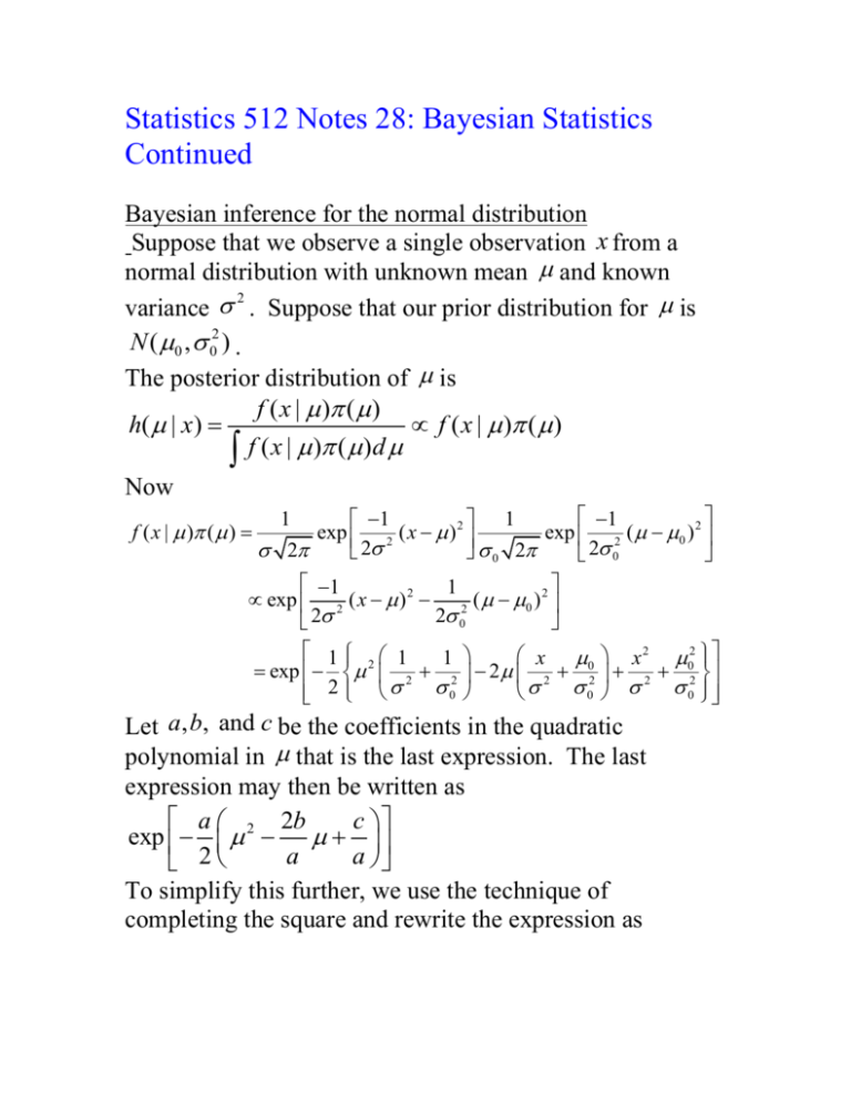
Statistics 512 Notes 28: Bayesian Statistics
Continued
Bayesian inference for the normal distribution
Suppose that we observe a single observation x from a
normal distribution with unknown mean  and known
2
variance  . Suppose that our prior distribution for  is
N ( 0 ,  02 ) .
The posterior distribution of  is
f ( x |  ) (  )
h(  | x ) 
 f ( x |  ) (  )
 f ( x |  ) ( )d 
Now
f ( x |  ) (  ) 
 1

1
 1
 1
exp  2 ( x   ) 2 
exp  2 (   0 ) 2 
 2
 2
  0 2
 2 0

 1

1
 exp  2 ( x   ) 2  2 (   0 ) 2 
2 0
 2

 1  2  1
 x 0  x 2 02 
1 
 exp      2  2   2   2  2   2  2 
0 
 0    0 
 2   

Let a, b, and c be the coefficients in the quadratic
polynomial in  that is the last expression. The last
expression may then be written as
 a
2b
c 
exp     2     
a
a 
 2
To simplify this further, we use the technique of
completing the square and rewrite the expression as
2
2

 a
b 
 a 2  c  b   

exp        exp 
    
a  

 2 
 2  a  a   

The second term does not depend on  and we thus have
that
2
 a
b 
h(  | x)  exp       
a  
 2 
This is the density of a normal random variable with mean
b
1
a and variance a .
Thus, the posterior distribution of  is normal with mean
x 0
 2
2
 0
1 
1
1

2
2

0
and variance
1
 12 
1
1 .

 2  02
Comments about role of prior in the posterior distribution:
The posterior mean is a weighted average of the prior mean
and the data, with weights proportional to the respective
precisions of the prior and the data, where the precision is
equal to 1/variance. If we assume that the experiment (the
observation of X ) is much more informative than the prior
2
2
distribution in the sense that    0 , then
 12   2
1  x
Thus, the posterior distribution of  is nearly normal with
2
mean x and variance  . This result illustrates that if the
prior distribution is quite flat relative to the likelihood, then
1. the prior distribution has little influence on the
posterior
2. the posterior distribution is approximately
proportional to the likelihood function.
On a heuristic level, the first point says that if one does not
have strong prior opinions, one’s posterior opinion is
mainly determined by the data one observes. Such a prior
distribution is often called a vague or noninformative prior.
Inference for sample of more than one observation
We now consider the posterior distribution when an iid
2
2
sample ( X 1 , , X n ) ~ N (  ,  ) is taken where  is known
2
and as before, we use the prior distribution N ( 0 ,  0 ) . As
before, the posterior distribution is proportional to
h(  | x1 , , xn )  f ( x1 , , xn |  ) (  ) .
From the independence of the X i ’s,
1
 1
exp
  2 2
 n (2 ) n / 2
Using the identity,
f ( x1 ,
, xn |  ) 
2
(
x


)
 i 1 i
 .
n
i1 ( xi   )2  i1 ( xi  x )2  n( x  )2
n
n
we obtain
f ( x1 ,
, xn |  ) 
1
 1
exp
  2 2
 n (2 ) n / 2

1

2
2
(
x

x
)
exp

(
x


)
i

 2 2 / n

i 1
n
Only the last term depends on  , so
1


h(  | x1 , , xn )  exp   2 ( x   ) 2   (  )
 2 / n

This posterior distribution can be evaluated in the same
way as the single observation case with x replacing x and
 2 / n replacing  2 . Thus, the posterior distribution is
normal with mean
0 nx

 02  2
1 
n
1

2
2

0
and variance
1
 12 
n
1

 2  02
2
For large values of n , 1  x and   n . Therefore, the
information in the sample largely determines the posterior
distribution for large samples.
2
1
Bayesian inference:
Point estimation: When faced with a decision, the Bayesian
wants to minimize the expected loss (i.e., maximize the
expected utility) of a decision rule under the prior
distribution  ( ) for  . In other words the Bayesian
chooses the decision rule d that minimizes the Bayes risk:
B(d )  E ( ) [ R( , d )] ,
i.e., the Bayesian chooses to use the Bayes rule for the
Bayesian’s prior distribution  ( )
As we showed in Notes 26, for point estimation with
squared error loss, the Bayes rule is to use the posterior
mean as the estimate.
Thus, for the above normal distribution setup, the
Bayesian’s estimate of  is
x 0
 2
2

0
1
1

 2  02
Interval estimation: A Bayesian version of a confidence
interval is called a credibility interval . A
100(1   )% credibility interval is an interval of the form
(0 ,1 ) , where
1

0
h( | x)d  1   .
, X n ) iid N (  ,  2 ) where  2 is
2
known and the prior distribution is N ( 0 ,  0 ) , the posterior
For example, for ( X 1 ,
 0 nx


2 2

1
0

N
,
n
1
n
1
distribution for  is 
 and a 95%


2 2 2 2 
0
0 

credibility interval for  is
0 nx

 02  2
1
 1.96
n
1
n
1


 2  02
 2  02
The frequentist confidence interval is not a probability
statement about  . The Bayesian credibility interval is a
statement about  . For the Bayesian, once the data x has
been observed, the interval is fixed and  is random.
Hypothesis testing: Consider testing H 0 :   0 vs.
H a :   0 . For the prior distribution, we need to put prior
probabilities on H 0 and H a and then put a prior on  under
H a . If we use the following 0-1 loss function
0 if   H i
L( , Hypothesis i chosen)= 
,
1 if   H i
the posterior risk is minimized by choosing the hypothesis
that is more probable under the posterior distribution.
Thus, the Bayes rule is to choose the hypothesis that is
more probable under the posterior distribution. Bayesian
hypothesis testing is a complex topic. The difficulty is that,
unlike in estimation problems, the prior is influential even
in large samples and so must be chosen carefully.
Chapter 15 from Rice, Mathematical Statistics and Data
Analysis provides another example of Bayesian inference
of Bayesian analysis for the binomial distribution.
Review of course
I. Three basic types of statistical inferences (Chapter 5):
1. Point estimation -- best estimate of parameter
2. Confidence intervals – how much uncertainty is there
in our estimate of the parameter.
3. Hypothesis testing – choose between two hypotheses
about the parameter.
II. Monte Carlo method for studying properties of
inference procedures and bootstrap method for constructing
confidence intervals based on Monte Carlo simulations
(Chapters 5.8-5.9)
III. Maximum likelihood method of making statistical
inferences and its properties (Chapter 6)
IV. Optimal point estimators: Cramer-Rao Lower Bound
(Chapter 6), sufficiency (Chapter 7.1-7.3), Rao-Blackwell
Theorem (Chapter 7.3).
V. Optimal hypothesis testing (Chapters 8.1-8.3).
VI. Decision theory (Chapter 7.1, my notes)
VII. Bayesian statistics (Chapter 11.1-11.2, my notes).