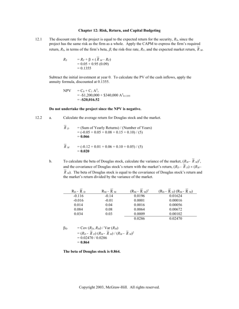
Chapter 12: Risk, Return, and Capital Budgeting
12.1
The discount rate for the project is equal to the expected return for the security, RS, since the
project has the same risk as the firm as a whole. Apply the CAPM to express the firm’s required
return, RS, in terms of the firm’s beta, , the risk-free rate, RF, and the expected market return, R M.
RS
= RF +   ( R M – RF)
= 0.05 + 0.95 (0.09)
= 0.1355
Subtract the initial investment at year 0. To calculate the PV of the cash inflows, apply the
annuity formula, discounted at 0.1355.
NPV
= C0 + C1 ATr
= -$1,200,000 + $340,000 A50.1355
= -$20,016.52
Do not undertake the project since the NPV is negative.
12.2
a.
b.
Calculate the average return for Douglas stock and the market.
RD
= (Sum of Yearly Returns) / (Number of Years)
= (-0.05 + 0.05 + 0.08 + 0.15 + 0.10) / (5)
= 0.066
RM
= (-0.12 + 0.01 + 0.06 + 0.10 + 0.05) / (5)
= 0.020
To calculate the beta of Douglas stock, calculate the variance of the market, (RM - R M)2,
and the covariance of Douglas stock’s return with the market’s return, (RD - R D)  (RM R M). The beta of Douglas stock is equal to the covariance of Douglas stock’s return and
the market’s return divided by the variance of the market.
RD - R D
-0.116
-0.016
0.014
0.084
0.034
D
RM - R M
-0.14
-0.01
0.04
0.08
0.03
(RM - R M)2
0.0196
0.0001
0.0016
0.0064
0.0009
0.0286
(RD - R D) (RM - R M)
0.01624
0.00016
0.00056
0.00672
0.00102
0.02470
= Cov (RD, RM) / Var (RM)
= (RD - R D) (RM - R M) / (RM - R M)2
= 0.02470 / 0.0286
= 0.864
The beta of Douglas stock is 0.864.
Copyright 2003, McGraw-Hill. All rights reserved.
12.3
Calculate the square root of the stock’s variance and the market’s variance to find the standard
deviation, , of each.
C
= (2C)1/2
= (0.004225)1/2
= 0.065
M
= (2M)1/2
= (0.001467)1/2
= 0.0383
Use the formula for beta:
C
= [Corr (RC, RM)  C] / M
= [(0.675) (0.065)] / (0.0383)
= 1.146
The beta of Ceramics Craftsman is 1.146.
12.4
a.
To compute the beta of Mercantile’s stock, divide the covariance of the stock’s return
with the market’s return by the market variance. Since those two values are provided in
the problem, the 13 quarterly returns of Mercantile’s stock and the market are not needed
for the calculation.
D
= Cov (RD, RM) / 2M
= (0.038711) / (0.038588)
= 1.0032
The beta of Mercantile Banking Corporation is 1.0032.
12.5
b.
The beta of the average stock is one. Since Mercantile’s beta is close to one, its stock has
approximately the same risk as the overall market.
a.
RL can have three values, 0.16, 0.18, or 0.20. The probability that RL takes one of these
values is the sum of the joint probabilities of the return pair, Prob(RL, RJ), that includes
the particular value of RL. For example, if RL is equal to 0.16, RJ will be either 0.16, 0.18,
or 0.22. The probability that RL is 0.16 and RJ is 0.16 is 0.10. The probability that RL is
0.16 and RJ is 0.18 is 0.06. The probability that RL is 0.16 and RJ is 0.22 is 0.04. Thus,
the probability that RL assumes a value 0.16 is 0.20 (=0.10 + 0.06 + 0.04). The same
procedure is used to calculate the probability that RL is 0.18 and the probability that RL is
0.20.
RL
0.16
0.18
0.20
b.
i.
Probability
0.20
0.60
0.20
The expected return on asset L is calculated by weighting each possible
return by its probability. Multiply each possible return, RL, by its probability, as
found in part (a).
RL
= [RL  Prob(RL)]
= (0.16)(0.20) + (0.18)(0.60) + (0.20) (0.20)
= 0.18
Copyright 2003, McGraw-Hill. All rights reserved.
The expected return on asset L is 18%.
ii.
The variance of asset L is the weighted sum of the squared differences between
the possible values of RL and the expected return on RL found in part (i). Weight
the squared differences by the probabilities of each value found in part (a).
2L
= [(RL - R L)2  Prob(RL)]
= (0.16 – 0.18)2 (0.20) + (0.18 – 0.18)2 (0.60) + (0.20 – 0.18)2 (0.20)
= 0.00016
The variance of asset L is 0.00016.
iii.
The standard deviation of asset L is the square root of the variance calculated in
part (ii).
L
= (2L)1/2
= (0.00016)1/2
= 0.01265
The standard deviation of asset L is 0.01265.
c.
Repeat the procedure used in part (a) to calculate the probability of each value of RJ.
RJ
0.16
0.18
0.20
0.22
0.24
d.
i.
Probability
0.10
0.20
0.40
0.20
0.10
The expected return on asset J is the weighted probability of each possible
return. Multiply each possible return, RJ, by the probability of each return found
in part (c).
RJ
= [RJ  Prob(RJ)]
= (0.16)(0.10) + (0.18)(0.20) + (0.20)(0.40) + (0.22)(0.20) +
(0.24)(0.10)
= 0.20
The expected return on asset J is 20%.
ii.
The variance of asset J is the weighted sum of the squared differences between
the possible values of RJ and the expected return on RJ found in part (i). Weight
the squared differences by the probabilities of each value found in part (c).
2J
= [(RJ - R J)2  Prob(RJ)]
= (0.16 – 0.20)2 (0.10) + (0.18 – 0.20)2 (0.20) + (0.20 – 0.20)2 (0.40) +
(0.22 – 0.20)2 (0.20) + (0.24 – 0.20)2 (0.10)
= 0.00048
The variance of asset J is 0.00048.
iii.
The standard deviation of asset J is the square root of the variance calculated in
part (ii).
Copyright 2003, McGraw-Hill. All rights reserved.
J
= (2J)1/2
= (0.00048)1/2
= 0.02191
The standard deviation of asset J is 0.02191.
d.
The covariance is the expected value of [(RL - R L) (RJ - R J)].
Cov (RL, RJ)
=  [(RL - R L)  (RJ - R J)  Prob (RL, RJ)]
= (0.16 – 0.18) (0.16 – 0.20) (0.10) + (0.16 – 0.18) (0.18 – 0.20) (0.06)
+ (0.16 – 0.18) (0.22 – 0.20) (0.04) + (0.18 – 0.18) (0.18 – 0.20) (0.12)
+ (0.18 – 0.18) (0.20 – 0.20) (0.36) + (0.18 – 0.18) (0.22 – 0.20) (0.12)
+ (0.20 – 0.18) (0.18 – 0.20) (0.02) + (0.20 – 0.18) (0.20 – 0.20) (0.04)
+ (0.20 – 0.18) (0.22 – 0.20) (0.04) + (0.20 – 0.18) (0.24 – 0.20) (0.10)
= 0.000176
The covariance of asset L’s return with asset J’s return is 0.000176.
The correlation coefficient of RL and RJ is the covariance divided by the standard
deviation of assets L and J.
Corr (RL, RJ)
= Cov (RL, RJ) / (L J)
= 0.000176 / (0.01265  0.02191)
= 0.635
The correlation coefficient of asset L and J is 0.635.
e.
Divide the product of the correlation coefficient and the standard deviation of asset J by
the standard deviation of the market, asset L, to calculate the beta for asset J.
J
= [Corr (RL, RJ)  J] / L
= [(0.635) (0.02191)] / (0.01265)
= 1.10
The beta of asset J is 1.10.
12.6
You are assuming that the new project’s risk is the same as the risk of the firm as a whole, and that
the firm is financed entirely with equity.
12.7
a.
Jang Cosmetics should use its stock beta in the evaluation of the project only if the risk of
the perfume project is the same as the risk of Jang Cosmetics as a whole.
b.
If the risk of the project is the same as the risk of the firm, use the firm’s stock beta.
Otherwise, Jang should use the beta of an all-equity firm that has similar risks as the
perfume project. An effective way to estimate the beta of the perfume project is to
average the betas of several all-equity, perfume-producing firms.
12.8
First, calculate the expected return on Compton’s stock.
RS
= [RS  Prob(RS)]
= (0.03) (0.1) + (0.08) (0.3) + (0.20) (0.4) + (0.15) (0.2)
= 0.137
Copyright 2003, McGraw-Hill. All rights reserved.
Calculate the expected return on Compton’s debt.
RB
= [RB  Prob(RB)]
= (0.08) (0.1) + (0.08) (0.3) + (0.1) (0.4) + (0.1) (0.2)
= 0.092
Calculate the expected return on the market.
RM
= [RM  Prob(RM)]
= (0.05) (0.1) + (0.1) (0.3) + (0.15) (0.4) + (0.2) (0.2)
= 0.135
Calculate the covariance of the stock’s return with the market’s return.
Cov (RS, RM)
=  [(RS - R S)  (RM - R M)  Prob]
= (0.03 – 0.137) (0.05 – 0.135) (0.1) + (0.08 – 0.137) (0.1 – 0.135)
(0.3) + (0.2 – 0.137) (0.15 – 0.135) (0.4) + (0.15 – 0.137) (0.2 – 0.135)
(0.2)
= 0.002055
Calculate the covariance of the debt’s return with the market’s return.
Cov (RB, RM)
=  [(RB - R B)  (RM - R M)  Prob]
= (0.08 – 0.092) (0.05 – 0.135) (0.1) + (0.08 – 0.092) (0.1 – 0.135)
(0.3) + (0.1 – 0.092) (0.15 – 0.135) (0.4) + (0.1 – 0.092) (0.2 – 0.135)
(0.2)
= 0.00038
Calculate the market variance.
2M
a.
= [(RM - R M)2  Prob(RM)]
= (0.05 – 0.135)2 (0.1) + (0.1 – 0.135)2 (0.3) + (0.15 – 0.135)2 (0.4) +
(0.2 – 0.135)2 (0.2)
= 0.002025
Calculate the beta of Compton Technology’s debt by dividing the covariance of the
debt’s return with the market’s return by the variance of the market.
B
= Cov (RB, RM) / 2M
= (0.00038) / (0.002025)
= 0.188
The beta of Compton Technology debt is 0.188.
b.
Calculate the beta of Compton Technology’s stock by dividing the covariance of the
stock’s return with the market’s return by the variance of the market.
S
= Cov (RS, RM) / 2M
= (0.002055) / (0.002025)
= 1.015
The beta of Compton Technology stock is 1.015.
Copyright 2003, McGraw-Hill. All rights reserved.
c.
Calculate the equity to value ratio [S / (S+B)] and the debt to value ratio [B / (S+B)] by
substitution.
B/S
B
= 0.5
= 0.5 S
[S / (S+B)]
= [S / (S + 0.5S)]
= [S / (1.5  S)]
= 1 / 1.5
= 0.667
[B / (S+B]
= [0.5  S / (S + 0.5  S)]
= [(0.5  S) / (1.5  S)]
=1/3
= 0.333
When there are no taxes, the asset beta is equal to the weighted average of the stock beta
and the debt beta.
Asset
= [S / (S+B)]  S + [B / (S+B)]  B
= (0.667) (1.015) + (0.333) (0.188)
= 0.740
The asset beta of Compton Technology is 0.740.
12.9
The discount rate for the projects should be lower that the rate implied by the security market line.
The security market line is used to calculate the cost of equity. The appropriate discount rate for
projects is the firm’s weighted average cost of capital. Since the firm’s cost of debt is generally
less that the firm’s cost of equity, the rate implied by the security market line will be too high.
12.10
Beta measures the responsiveness of a security's returns to movements in the market. Beta is
determined by the cyclicality of a firm's revenues. This cyclicality is magnified by the firm's
operating and financial leverage.
a.
Revenues. The cyclicality of a firm's sales is an important factor in determining beta. In
general, stock prices will rise when the economy expands and will fall when the economy
contracts. As we said above, beta measures the responsiveness of a security's returns to
movements in the market. Therefore, firms whose revenues are more responsive to
movements in the economy will generally have higher betas than firms with less-cyclical
revenues.
b.
Operating leverage. Operating leverage is the percentage change in earnings before interest
and taxes (EBIT) for a percentage change in sales. A firm with high operating leverage will
have greater fluctuations in EBIT for a change in sales than a firm with low operating
leverage. In this way, operating leverage magnifies the cyclicality of a firm's revenues,
leading to a high beta.
c.
Financial leverage. Financial leverage arises from the use of debt in the firm's capital
structure. A levered firm must make fixed interest payments regardless of its revenues. The
effect of financial leverage on beta is analogous to the effect of operating leverage on beta.
Fixed interest payments cause the percentage change in net income to be greater than the
percentage change in EBIT, magnifying the cyclicality of a firm's revenues. Thus, returns on
highly-levered stocks should be more responsive to movements in the market than the returns
on stocks with little or no debt in their capital structure.
Copyright 2003, McGraw-Hill. All rights reserved.
12.11
a.
Apply the CAPM to calculate the cost of equity.
rS
= RF + S  ( R M – RF)
= 0.06 + 1.15 (0.1)
= 0.175
The cost of equity is 17.5%.
b.
To calculate the weighted average cost of capital for the project, r WACC, first determine
the cost of debt, rB. Use the cost of equity, rS, calculated in part (a).
rB
= RF + B  ( R M – RF)
= 0.06 + 0.3 (0.1)
= 0.09
rS
= 0.175
Next, calculate the weighted average cost of capital. To determine the proper weights,
express the firm’s proportion of debt in terms of the firm’s proportion of equity. Solve
for the equity to value ratio [S / (S+B)] and the debt to value ratio [B / (S+B)].
B/S
B
= 0.25
= 0.25 S
[S / (S+B)]
= [S / (S + 0.25S)]
= [S / (1.25  S)]
= 1 / 1.25
= 0.80
[B / (S+B]
= [0.25  S / (S + 0.25  S)]
= [(0.25  S) / (1.25  S)]
=1/5
= 0.20
Interest on debt is tax deductible at the corporate level, which leads to tax benefits for the
firm. Multiply the cost of debt, rB, by (1 - TC), to include the tax benefit created by the
interest tax shield. The tax benefit of debt will lower the firm’s overall cost of capital.
rWACC
= [S / (S+B)]  rS + [B / (S+B)]  rB  (1 – TC)
= (0.80) (0.175) + (0.20) (0.09) (0.65)
= 0.1517
The weighted average cost of capital is 15.17%.
12.12
a.
Apply the CAPM to estimate Adobe Online’s cost of equity, RS. The following equation
expresses the firm’s required return, RS, in terms of the firm’s beta, S, the risk-free rate,
RF, and the market return, R M.
RS
= RF +   ( R M – RF)
= 0.07 + 1.29 (0.13 – 0.07)
= 0.1474
Adobe Online’s cost of equity is 14.74%.
Copyright 2003, McGraw-Hill. All rights reserved.
b.
Use the debt-to-equity ratio to determine the weighted average cost of capital. Calculate
the equity to value ratio [S / (S+B)] and the debt to value ratio [B / (S+B)] by
substitution.
B/S
B
= 1.0
= S
[S / (S+B)]
= [S / (S + S)]
= [S / (2  S)]
=1/2
= 0.5
[B / (S+B]
= [1.0  S / (S + 1.0  S)]
= [(S) / (2  S)]
=1/2
= 0.5
Remember that interest on debt is tax deductible at the corporate level, which will lower
the firm’s overall cost of capital. Multiply the cost of debt, r B, by (1 - TC) to include the
interest tax shield in the weighted average cost of capital.
rWACC
= [S / (S+B)]  rS + [B / (S+B)]  rB  (1 – TC)
= (0.5) (0.1474) + (0.5) (0.07) (1 – 0.35)
= 0.09645
The weighted average cost of capital is 9.645%.
12.13
Use the market value of debt to compute the weighted average cost of capital. To calculate the
market value of the debt, multiply the book value of Luxury’s debt by 120 percent.
B
= $60,000,000  1.2
= $72,000,000
The market value of Luxury’s stock is equal to the number of shares outstanding multiplied by the
market price per share.
S
= 5,000,000  $20
= $100,000,000
The value of the firm is the market value of Luxury’s debt plus the market value of Luxury’s
stock.
V
=B+S
= $72,000,000 + $100,000,000
= $172,000,000
Calculate the debt-to-value and equity-to-value ratios. These ratios will be used to compute the
weighted average cost of capital.
B / (S + B)
= $72,000,000 / $172,000,000
= 0.4186
S / (S + B)
= $100,000,000 / $172,000,000
= 0.5814
Copyright 2003, McGraw-Hill. All rights reserved.
Use the cost of debt and cost of equity, 12 percent and 18 percent, respectively, and the weights
calculated above, to determine the weighted average cost of capital. Remember that interest on
debt is tax deductible at the corporate level, which will lower the firm’s overall cost of capital.
Multiply the cost of debt, rB, by (1 - TC) to include the interest tax shield in the weighted average
cost of capital.
rWACC
= [S / (S+B)]  rS + [B / (S+B)]  rB  (1 – TC)
= (0.5814) (0.18) + (0.4186) (0.12) (0.75)
= 0.1423
The weighted average cost of capital for Luxury Porcelain Company is 14.23%.
12.14
Use the market value of debt to calculate the weighted average cost of capital. To compute the
market value of the debt, multiply the book value of First Data’s debt by 95 percent.
B
= $180,000,000  0.95
= $171,000,000
The market value of First Data Co.’s stock is equal to the number of shares outstanding multiplied
by the market price per share.
S
= 20,000,000  $25
= $500,000,000
The value of the firm is the market value of First Data Co.’s debt plus the market value of the
stock.
V
=B+S
= $171,000,000 + $500,000,000
= $671,000,000
Calculate the debt-to-value and equity-to-value ratios. These ratios will be used to compute the
weighted average cost of capital.
B / (S + B)
= $171,000,000 / $671,000,000
= 0.2548
S / (S + B)
= $500,000,000 / $671,000,000
= 0.7452
Apply the weighted average cost of capital formula, using the cost of debt and cost of equity given
in the problem, 10 percent and 20 percent, respectively. Remember that interest on debt is tax
deductible at the corporate level, which will lower the firm’s overall cost of capital. Multiply the
cost of debt, rB, by (1 - TC) to include the interest tax shield in the weighted average cost of
capital.
rWACC
= [S / (S+B)]  rS + [B / (S+B)]  rB  (1 – TC)
= (0.7452) (0.20) + (0.2548) (0.10) (0.60)
= 0.1643
The weighted average cost of capital for First Data Co. is 16.43%.
12.15
The appropriate discount rate for the project is the weighted average cost of capital. Use the debtto-equity ratio to calculate the weighted average cost of capital. Determine the equity to value
ratio [S / (S+B)] and the debt to value ratio [B / (S+B)] by substitution.
Copyright 2003, McGraw-Hill. All rights reserved.
B/S
B
= 0.75
= 0.75  S
[S / (S+B)]
= [S / (S + 0.75  S)]
= [S / (1.75  S)]
= 1 / 1.75
= 0.5714
[B / (S+B]
= [(0.75  S) / (S + 0.75  S)]
= [(0.75  S) / (1.75  S)]
= 0.75 / 1.75
= 0.4286
Remember that interest on debt is tax deductible at the corporate level, which will lower the firm’s
overall cost of capital. Multiply the cost of debt, rB, by (1 - TC) to include the interest tax shield in
the weighted average cost of capital.
rWACC
= [S / (S+B)]  rS + [B / (S+B)]  rB  (1 – TC)
= (0.5714) (0.15) + (0.4286) (0.09) (0.65)
= 0.1108
To calculate the NPV of the project, subtract the initial (year 0) outlay. Next, apply the annuity
formula, discounted at the weighted average cost of capital, to calculate the PV of the cash
inflows.
NPV
= C0 + C1 ATr
= -$25,000,000 + $7,000,000 A50.1108
= $819,299.04
Since the project has a positive NPV, $819,299.04, the company should accept the project.
12.16
The correct discount rate for the project is the weighted average cost of capital. Since the debt-toequity ratio is equal to one, the debt-to-value and equity-to-value ratios will be equal to 0.5.
Remember that interest on debt is tax deductible at the corporate level, which will lower the firm’s
overall cost of capital. Multiply the cost of debt, rB, by (1 - TC) to include the interest tax shield in
the weighted average cost of capital.
rWACC
= [S / (S+B)]  rS + [B / (S+B)]  rB  (1 – TC)
= (0.5) (0.28) + (0.5) (0.1) (0.65)
= 0.1725
To calculate the NPV of the project, subtract the initial (year 0) outlay. Next, apply the annuity
formula, discounted at the weighted average cost of capital, to calculate the PV of the cash
inflows. Remember to adjust the pre-tax annual earnings of $600,000 for taxes.
NPV
= C0 + (1 – Tc) C1 ATr
= -$1,000,000 + (0.65) $600,000 A50.1725
= $240,608.65
The NPV of the project is $240,608.65. The firm should accept the project.
Copyright 2003, McGraw-Hill. All rights reserved.