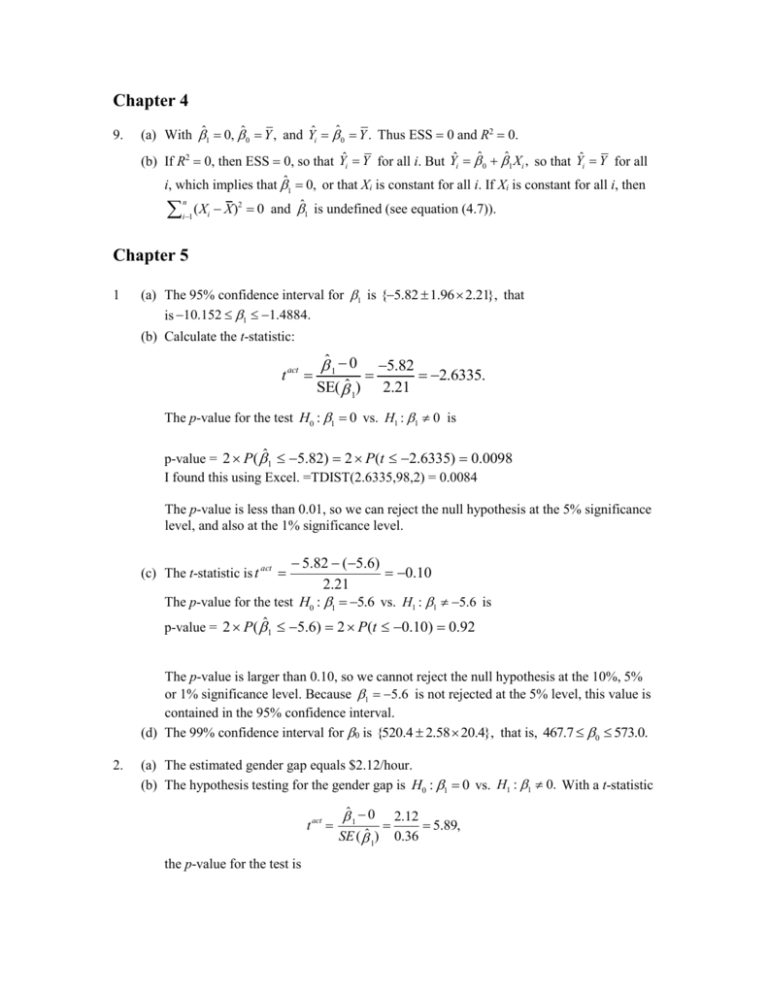
Chapter 4
9.
(a) With ˆ1  0, ˆ0  Y , and Yˆi  ˆ0  Y . Thus ESS  0 and R2  0.
(b) If R2  0, then ESS  0, so that Yˆi  Y for all i. But Yˆi  ˆ0  ˆ1 Xi , so that Yˆi  Y for all
i, which implies that ˆ  0, or that Xi is constant for all i. If Xi is constant for all i, then
1

n
i1
( Xi  X)  0 and ̂1 is undefined (see equation (4.7)).
2
Chapter 5
1
(a) The 95% confidence interval for 1 is {582  196  221}, that
is 10152  1  14884.
(b) Calculate the t-statistic:
t act 
ˆ 1  0 582

 26335
SE( ˆ 1) 221
The p-value for the test H0  1  0 vs. H1  1  0 is
p-value = 2  P( ˆ1  5.82)  2  P(t  2.6335)  0.0098
I found this using Excel. =TDIST(2.6335,98,2) = 0.0084
The p-value is less than 0.01, so we can reject the null hypothesis at the 5% significance
level, and also at the 1% significance level.
 5.82  (5.6)
 0.10
2.21
The p-value for the test H0 : 1  5.6 vs. H1 : 1  5.6 is
p-value = 2  P( ˆ  5.6)  2  P(t  0.10)  0.92
(c) The t-statistic is t act 
1
The p-value is larger than 0.10, so we cannot reject the null hypothesis at the 10%, 5%
or 1% significance level. Because 1  5.6 is not rejected at the 5% level, this value is
contained in the 95% confidence interval.
(d) The 99% confidence interval for 0 is {520.4  2.58  20.4}, that is, 467.7  0  573.0.
2.
(a) The estimated gender gap equals $2.12/hour.
(b) The hypothesis testing for the gender gap is H0  1  0 vs. H1  1  0. With a t-statistic
t act 
the p-value for the test is
ˆ 1  0 2.12

 5.89
SE ( ˆ 1) 036
p-value = 2  P( ˆ1  2.12)  2  P(t  5.89)  6.88038E - 09  0.000 (to four decimal
places)
=TDIST(5.89,528,2) using excel
The p-value is less than 0.01, so we can reject the null hypothesis that there is no gender
gap at a 1% significance level.
(c) The 95% confidence interval for the gender gap 1 is {212  196  036}, that is,
141  1  2.83.
(d) The sample average wage of women is ˆ0  $1252/hour. The sample average wage of
men is ˆ 0  ˆ 1  $12.52  $2.12  $14.64/hour.
(e) The binary variable regression model relating wages to gender can be written as either
Wage  0  1Male  ui 
or
Wage   0   1Female  vi 
In the first regression equation, Male equals 1 for men and 0 for women;  0 is the
population mean of wages for women and  0  1 is the population mean of wages for
men. In the second regression equation, Female equals 1 for women and 0 for men;  0
is the population mean of wages for men and  0   1 is the population mean of wages
for women. We have the following relationship for the coefficients in the two regression
equations:
 0   0  1 
 0   1  0 
Given the coefficient estimates ̂ 0 and ˆ 1 , we have
ˆ 0  ˆ 0  ˆ 1  14.64
ˆ 1  ˆ 0  ˆ 0   ˆ 1  212
Due to the relationship among coefficient estimates, for each individual observation, the
OLS residual is the same under the two regression equations: uˆ i  vˆ i. Thus the sum of
squared residuals, SSR   i 1 uˆ i2, is the same under the two regressions. This implies
n
2
2
SSR
that both SER   SSR
n 1  and R  1  TSS are unchanged.
1
In summary, in regressing Wages on Female, we will get
Wages  14.64  212 Female
R2  006 SER  4.2
3.
The 99% confidence interval is 1.5  {3.94  2.58  0.31) or 4.71 lbs  WeightGain  7.11
lbs.
4.
(a) 3.13  1.47  16  $20.39 per hour
(b) The wage is expected to increase from $14.51 to $17.45 or by $2.94 per hour.
(c) The increase in wages for college education is 1  4. Thus, the counselor’s assertion is
that
2.50
1  10/4  2.50. The t-statistic for this null hypothesis is t  1.470.07
 14.71, which has a
p-value of 0.00. Thus, the counselor’s assertion can be rejected at the 1% significance
level. A 95% confidence for 1  4 is 4  (1.47  1.97  0.07) or $5.33  Gain  $6.43.
7.
3.2
(a) The t-statistic is 1.5
 2.13 with a p-value of 0.034; since the p-value is less than 0.05,
the null hypothesis is rejected at the 5% level. This is
2  P( ˆ1  3.2)  2  P(t  2.13)  0.034
(=TDIST(2.13,248,2) in excel0
(b) 3.2  1.96  1.5  3.2  2.94
(c) Yes. If Y and X are independent, then 1  0; but this null hypothesis was rejected at the
5% level in part (a).
(d) 1 would be rejected at the 5% level in 5% of the samples; 95% of the confidence
intervals would contain the value 1  0.
8.
(a) 43.2  2.05  10.2 or 43.2  20.91, where 2.05 is the 5% two-sided critical value from
the t28 distribution.
(b) The t-statistic is t act  61.57.455  0.88, which is less (in absolute value) than the critical
value of 2.05, thus, the null hypothesis is not rejected at the 5% level.
(c) The one sided 5% critical value is 1.70; tact is less than this critical value, so that the null
hypothesis is not rejected at the 5% level.
14. derive the OLS estimator when the model doesn’t have an intercept
 uˆ
2
i
  (Yi  ˆX i ) 2
SSR
 2 (Yi  ˆX i ) X i  0
ˆ
 (Y  ˆX ) X  0
 Y X   ˆX  0
 Y X  ˆ  X  0
 Y X  ˆ  X
Y X
ˆ 
X
i
i
i
2
i
i
i
i
i
2
i
i
i
2
i
i
i
2
i
Chapter 6
1.
By equation (6.15) in the text, we know
R2  1 
n 1
(1  R2 ).
n  k 1
Thus, that values of R2 are 0.175, 0.189, and 0.193 for columns (1)–(3).
2.
(a) Workers with college degrees earn $5.46/hour more, on average, than workers with only
high school degrees.
(b) Men earn $2.64/hour more, on average, than women.
5.
(a) $23,400 (recall that Price is measured in $1000s).
(b) In this case BDR  1 and Hsize  100. The resulting expected change in price is 23.4 
0.156  100  39.0 thousand dollars or $39,000.
(c) The loss is $48,800.
(d) From the text R2  1  nnk11 (1  R2 ), so R2  1  nnk11 (1  R2 ), thus, R2  0.727.
6.
(a) There are other important determinants of a country’s crime rate, including demographic
characteristics of the population.
(b) Suppose that the crime rate is positively affected by the fraction of young males in the
population, and that counties with high crime rates tend to hire more police. In this case,
the size of the police force is likely to be positively correlated with the fraction of young
males in the population leading to a positive value for the omitted variable bias so that
ˆ1  1.
Chapter 7
2. a) Yes, the variable COLLEGE has a t-stat of 5.46/0.21 = 26.00, which is clearly greater than the
critical t value of 2.57 at a 1% level of significance.
A 95% confidence interval would be 5.46 ±1.96*(0.21) = 5.46 ± 0.4116 = [5.05 , 5.87]
4.
(a) The F-statistic testing the coefficients on the regional regressors are zero is 6.10. The
1% critical value (from the F3,  distribution) is 3.78. Because 6.10 > 3.78, the regional
effects are significant at the 1% level.
The F stat can be calculated using SSRR and SSRU *or*
See page 231 F 
R2R and R2U
(0.194  0.190) 3
 6.605
(1  0.194) /( 4000  6  1)
(b) The expected difference between Juanita and Molly is (X6,Juanita  X6,Molly)  6  6. Thus
a 95% confidence interval is 0.27  1.96  0.26.
(c) The expected difference between Juanita and Jennifer is (X5,Juanita  X5,Jennifer)  5 
(X6,Juanita  X6,Jennifer)  6  5  6. A 95% confidence interval could be contructed using
the general methods discussed in Section 7.3. In this case, an easy way to do this is to omit
Midwest from the regression and replace it with X5  West. In this new regression the
coefficient on South measures the difference in wages between the South and the Midwest,
and a 95% confidence interval can be computed directly.
6.
In isolation, these results do imply gender discrimination. Gender discrimination means that
two workers, identical in every way but gender, are paid different wages. Thus, it is also
important to control for characteristics of the workers that may affect their productivity
(education, years of experience, etc.) If these characteristics are systematically different
between men and women, then they may be responsible for the difference in mean wages. (If
this were true, it would raise an interesting and important question of why women tend to
have less education or less experience than men, but that is a question about something other
than gender discrimination.) These are potentially important omitted variables in the
regression that will lead to bias in the OLS coefficient estimator for Female. Since these
characteristics were not controlled for in the statistical analysis, it is premature to reach a
conclusion about gender discrimination.
7.
(a) The t-statistic is 0.485
 0.186  1.96. Therefore, the coefficient on BDR is not
2.61
statistically significantly different from zero.
(b) The coefficient on BDR measures the partial effect of the number of bedrooms holding
house size (Hsize) constant. Yet, the typical 5-bedroom house is much larger than the
typical 2-bedroom house. Thus, the results in (a) says little about the conventional
wisdom.
(c) The 99% confidence interval for effect of lot size on price is 2000  [.002  2.58 
.00048] or 1.52 to 6.48 (in thousands of dollars).
(d) Choosing the scale of the variables should be done to make the regression results easy to
read and to interpret. If the lot size were measured in thousands of square feet, the
estimate coefficient would be 2 instead of 0.002.
(e) The 10% critical value from the F2, distribution is 2.30. Because 0.08 < 2.30, the
coefficients are not jointly significant at the 10% level.
Chapter 8
2.
(a) According to the regression results in column (1), the log of price is expected to increase
0.00042 x 500 = 0.21, meaning price is expected to increase by 21% with an additional
500 square feet and other factors held constant. The 95% confidence interval for the
change is 500  (0.00042  1.96  0.000038)  [.17276 to .24724].or 17.3% to 24.7%
(b) Because the regressions in columns (1) and (2) have the same dependent variable,
R2 can be used to compare the fit of these two regressions. The log-log regression in
column (2) has the higher R 2 , so it is better so use ln(Size) to explain house prices.
(c) The house price is expected to increase by 7.1% (the log of price is expected to change
by 0.071
(d) The house price is expected to increase by 0.36% (the log of price is expected to change
by 0.0036) with an additional bedroom while other factors are held constant. The effect
is not statistically significant at a 5% significance level: | t |  0.0036
 0.09730  1.96.
0.037
Note that this coefficient measures the effect of an additional bedroom holding the size
of the house constant.
(e) The quadratic term ln(Size)2 is not important. The coefficient estimate is not statistically
significant at a 5% significance level: | t |  0.0078
 0.05571  1.96.
0.14
(f) The house price is expected to increase by 7.1% when a swimming pool is added to a
house without a view and other factors are held constant. The house price is expected to
increase by 7.32% = 7.1% + .22%
 ln PRICE  ˆ pool  ˆ poolviewVIEW  0.071  0.0022(1)  0.0732
So a 7.32% increase in price. when a swimming pool is added to a house with a view and
other factors are held constant. The difference in the expected percentage change in
price is 0.22%. The difference is not statistically significant at a 5% significance level:
| t |  0.0022
 0.022  1.96.
0.10