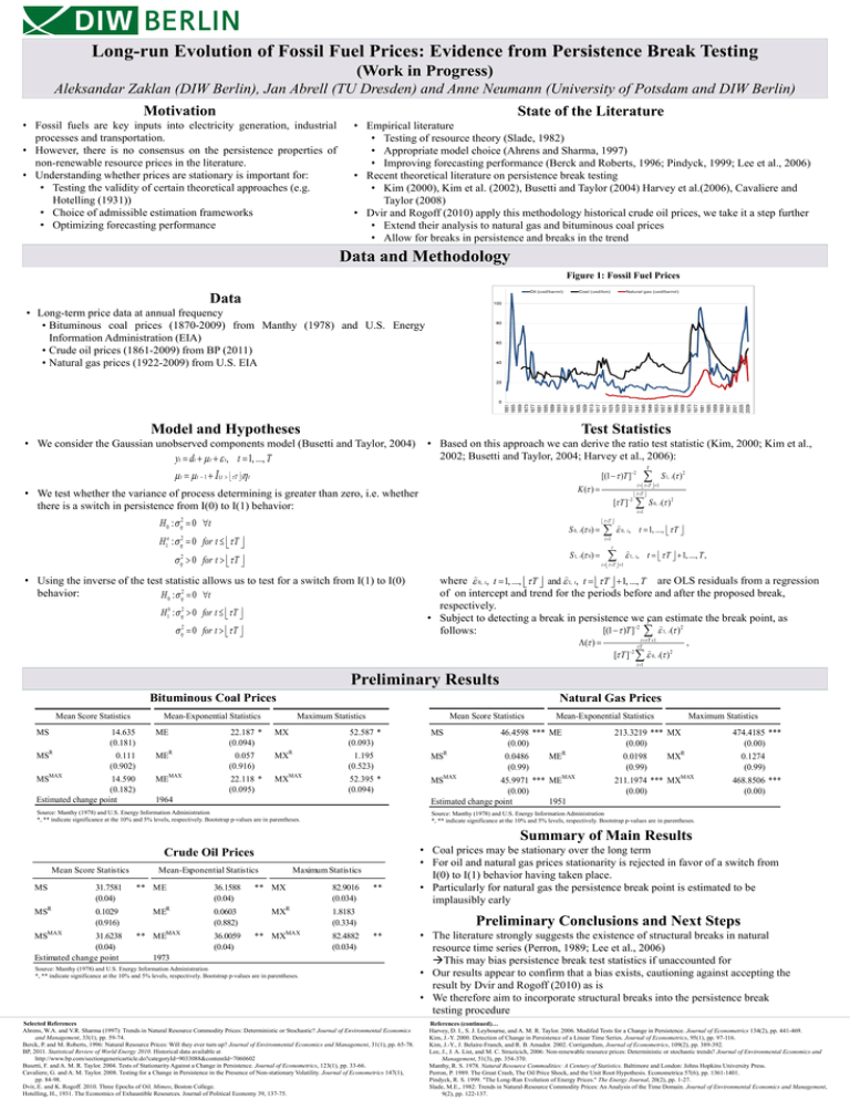
Long-run Evolution of Fossil Fuel Prices: Evidence from Persistence Break Testing
(Work in Progress)
Aleksandar Zaklan (DIW Berlin), Jan Abrell (TU Dresden) and Anne Neumann (University of Potsdam and DIW Berlin)
Motivation
State of the Literature
• Fossil fuels are key inputs into electricity generation, industrial
processes and transportation.
• However, there is no consensus on the persistence properties of
non-renewable resource prices in the literature.
• Understanding whether prices are stationary is important for:
• Testing the validity of certain theoretical approaches (e.g.
Hotelling (1931))
• Choice of admissible estimation frameworks
• Optimizing forecasting performance
• Empirical literature
• Testing of resource theory (Slade, 1982)
• Appropriate model choice (Ahrens and Sharma, 1997)
• Improving forecasting performance (Berck and Roberts, 1996; Pindyck, 1999; Lee et al., 2006)
• Recent theoretical literature on persistence break testing
• Kim (2000), Kim et al. (2002), Busetti and Taylor (2004) Harvey et al.(2006), Cavaliere and
Taylor (2008)
• Dvir and Rogoff (2010) apply this methodology historical crude oil prices, we take it a step further
• Extend their analysis to natural gas and bituminous coal prices
• Allow for breaks in persistence and breaks in the trend
Data and Methodology
Figure 1: Fossil Fuel Prices
Data
• Long-term price data at annual frequency
• Bituminous coal prices (1870-2009) from Manthy (1978) and U.S. Energy
Information Administration (EIA)
• Crude oil prices (1861-2009) from BP (2011)
• Natural gas prices (1922-2009) from U.S. EIA
Model and Hypotheses
Test Statistics
• We consider the Gaussian unobserved components model (Busetti and Taylor, 2004)
yt  dt   t   t , t  1, ..., T
t  t  1  1
• Based on this approach we can derive the ratio test statistic (Kim, 2000; Kim et al.,
2002; Busetti and Taylor, 2004; Harvey et al., 2006):



[(1   )T ]2
( t   T  ) t
K ( ) 
• We test whether the variance of process determining is greater than zero, i.e. whether
there is a switch in persistence from I(0) to I(1) behavior:
[ T ]2
H 0 :   0 t
S 0, t ( 0) 
H1a : 2  0 for t   T 
 0T 

0, i
i 1
S 1, t ( 0) 
  0 for t   T 
2

t


i   0T  1
• Using the inverse of the test statistic allows us to test for a switch from I(1) to I(0)
behavior:
H 0 : 2  0 t
H :   0 for t   T 
2

  0 for t   T 
2

S 1, i( ) 2
i   0T  1
 0T 

S 0, i ( ) 2
i 1
2

b
1
T
, t  1, ...,  T 
 1, i, t   T   1, ..., T ,
where  0, t, t  1, ...,  T  and  1, t, t   T   1, ..., T are OLS residuals from a regression
of on intercept and trend for the periods before and after the proposed break,
respectively.
• Subject to detecting a break in persistence we Tcan estimate the break point, as
2
2
[(1


)
T
]

1,
i
(

)
follows:

( ) 
i  T 1
T
[ T ]2   0, i ( )2
,
i 1
Preliminary Results
Bituminous Coal Prices
Mean Score Statistics
Mean-Exponential Statistics
Natural Gas Prices
Mean Score Statistics
Maximum Statistics
MS
14.635
(0.181)
ME
22.187 *
(0.094)
MX
52.587 *
(0.093)
MS
MSR
0.111
(0.902)
MER
0.057
(0.916)
MXR
1.195
(0.523)
MSR
MEMAX
22.118 *
(0.095)
MXMAX
52.395 *
(0.094)
MSMAX
MSMAX
14.590
(0.182)
Estimated change point
1964
Source: Manthy (1978) and U.S. Energy Information Administration
*, ** indicate significance at the 10% and 5% levels, respectively. Bootstrap p-values are in parentheses.
*, ** indicate significance at the 10% and 5% levels, respectively. Bootstrap p-values are in
parentheses.
Crude Oil Prices
Mean Score Statistics
Mean-Exponential Statistics
Maximum Statistics
MS
31.7581
** ME
36.1588
** MX
82.9016
**
(0.04)
Mean Score(0.04)
Statistics
Mean-Exponential
Statistics
Maximum (0.034)
Statistics
MSR
0.1029
MER
0.0603
MXR
1.8183
MS
18.7789 * ME
29.8162 ** MX
68.4125 **
(0.916)
(0.882)
(0.334)
(0.059)
(0.027)
(0.027)
MAX
MAX
MAX
MS
31.6238
**
ME
36.0059
**
MX
82.4882
**
R
R
MS
0.1294
ME
0.0676
MXR
1.3667
(0.04)(0.921)
(0.04)(0.929)
(0.034)
(0.530)
Estimated
1973MAX
MAX change point
MS
18.7187 * ME
29.7207 ** MXMAX
68.1542 **
Source: Manthy (1978) and U.S. Energy Information Administration
(0.060)
(0.027)are in parentheses.
(0.027)
*, ** indicate significance at the
10% and 5% levels, respectively. Bootstrap p-values
Estimated change point
1964
Selected References
Ahrens, W.A. and V.R. Sharma (1997): Trends in Natural Resource Commodity Prices: Deterministic or Stochastic? Journal of Environmental Economics
and Management, 33(1), pp. 59-74.
Berck, P. and M. Roberts, 1996: Natural Resource Prices: Will they ever turn up? Journal of Environmental Economics and Management, 31(1), pp. 65-78.
BP, 2011. Statistical Review of World Energy 2010. Historical data available at
http://www.bp.com/sectiongenericarticle.do?categoryId=9033088&contentId=7060602
Busetti, F. and A. M. R. Taylor. 2004. Tests of Stationarity Against a Change in Persistence. Journal of Econometrics, 123(1), pp. 33-66.
Cavaliere, G. and A. M. Taylor. 2008. Testing for a Change in Persistence in the Presence of Non-stationary Volatility. Journal of Econometrics 147(1),
pp. 84-98.
Dvir, E. and K. Rogoff. 2010. Three Epochs of Oil. Mimeo, Boston College.
Hotelling, H., 1931. The Economics of Exhaustible Resources. Journal of Political Economy 39, 137-75.
Mean-Exponential Statistics
46.4598 *** ME
(0.00)
0.0486
(0.99)
MER
45.9971 *** MEMAX
(0.00)
Estimated change point
1951
Maximum Statistics
213.3219 *** MX
(0.00)
0.0198
(0.99)
474.4185 ***
(0.00)
MXR
211.1974 *** MXMAX
(0.00)
0.1274
(0.99)
468.8506 ***
(0.00)
Source: Manthy (1978) and U.S. Energy Information Administration
*, ** indicate significance at the 10% and 5% levels, respectively. Bootstrap p-values are in parentheses.
Summary of Main Results
• Coal prices may be stationary over the long term
• For oil and natural gas prices stationarity is rejected in favor of a switch from
I(0) to I(1) behavior having taken place.
• Particularly for natural gas the persistence break point is estimated to be
implausibly early
Preliminary Conclusions and Next Steps
• The literature strongly suggests the existence of structural breaks in natural
resource time series (Perron, 1989; Lee et al., 2006)
This may bias persistence break test statistics if unaccounted for
• Our results appear to confirm that a bias exists, cautioning against accepting the
result by Dvir and Rogoff (2010) as is
• We therefore aim to incorporate structural breaks into the persistence break
testing procedure
References (continued)…
Harvey, D. I., S. J. Leybourne, and A. M. R. Taylor. 2006. Modifed Tests for a Change in Persistence. Journal of Econometrics 134(2), pp. 441-469.
Kim, J.-Y. 2000. Detection of Change in Persistence of a Linear Time Series. Journal of Econometrics, 95(1), pp. 97-116.
Kim, J.-Y., J. Belaire-Franch, and R. B. Amador. 2002. Corrigendum, Journal of Econometrics, 109(2), pp. 389-392.
Lee, J., J. A. List, and M. C. Strazicich, 2006: Non-renewable resource prices: Deterministic or stochastic trends? Journal of Environmental Economics and
Management, 51(3), pp. 354-370.
Manthy, R. S. 1978. Natural Resource Commodities: A Century of Statistics. Baltimore and London: Johns Hopkins University Press.
Perron, P. 1989. The Great Crash, The Oil Price Shock, and the Unit Root Hypothesis. Econometrica 57(6), pp. 1361-1401.
Pindyck, R. S. 1999. "The Long-Run Evolution of Energy Prices." The Energy Journal, 20(2), pp. 1-27.
Slade, M.E., 1982: Trends in Natural-Resource Commodity Prices: An Analysis of the Time Domain. Journal of Environmental Economics and Management,
9(2), pp. 122-137.