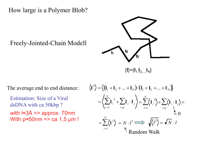
How large is a Polymer Blob?
Freely-Jointed-Chain Modell
{l}={l1,l2,...,lN}
The average end to end distance:
Estimation: Size of a Viral
dsDNA with ca 50kbp ?
with l≈3Å => approx. 70nm
With p≈50nm => ca 1,5 µm !
l
2
 l1  l 2  ...  l N  l1  l2 ...  l N 
N

l
i 1
2
i
N
 l i  l j   l i 2   l i  l j 
i j
i 1
i j
0
N
  l 2  N  l2
i 1
l
2
Random Walk

N l
The excluded Volume
• The simple model of a random walk resulted
for the end to end distance oft the polymer blob:
r2  N  l2
• Problem: The polymer cannot occupy the same space. Thus the average quadratic
end to end distance should be bigger.
• Flory solved the problem with a simple heuristic argument:
If two monomers overlap, they repell each other. The Probability that 2 monomers
occupy the same space increases with the concentration squared
Energy Density:
W  vkBT cm
W  vkBT 
N
2
r2
E Ausschluß  W 
Gaub/WS 2006
cm 
2
N
r
2
3
The average end to end
distance is used as measure
for the radius of the
polymers.
6
r2
3
 vkB T 
BPM §1.4.2
N2
r
2
3
2
• The energy for the excluded volume drives the polymer blob apart. This force has
to be balanced by an entropic force which wants to keep the blob together:
EA usschluß  W 
FAusschluß 
E Ausschluß

Fentr
3kT
2 
Nl
1
2 
l
Gaub/WS 2006
r
2
r
r
2
3
 vkB T 
r
2
r
r
2
5
 v  N
3
5
3
2
N2
r
2
4
(von FJC Model)
N2
 vkBT 3
2
r
 vkB T  3
3kT

2 
N l
2
N2
r2
!
4
0
3
BPM
N §1.4.2
In contrast to the FJC Model
r
2
N
0.5
3
Java-Simulation Self-avoiding Random Walk
http://polymer.bu.edu/java/java/saw/sawapplet.html
The Worm-Like-Chain Model for semiflexible Polymers
s
s

A measure for the stiffness of a polymer is the persistence length Lp, which measures
at which length s=Lp the orientation  and s are not correlated any more.
A measure for the correlation of the orientation oBdA
is the following average value:
f(s)  cos (s)  (0)
 cos (s)
1
1
cos( ) d 2 O(d 4 )   sin(  ) d  cos( ) d 2
2
2
1
1
2
2
  f (s) d
  sin(  )  d  cos( )  d
2
2
df   sin(  ) d 
=0
Gaub/WS 2006
d 2
df
1
  BPM
f(s)§1.4.2
   ds
 ds 
ds
2
5
Calculation: Energy change of a beam of length
s, if it is bent by the angle 
Local Bending Radius
dU  M  d
E
mit M  I
R

EI 1
dU 
 d  s

R R

U 

0
d 1

ds R
R

EI 1 

 d  s
R R 
1
R0
  R  s
d 2
1 EI
EI 1 
1
 d  s 
EI    s
2  s 
 ds 
2 R0
R R 
2

s
d 2 2 U
  
 ds  EI  s
d 2
df
1
  f(s)    ds
 ds 
ds
2
d 2 2 U
  
 ds  EI  s
df
1
kT
  f(s)
Äquipartition Theorem
ds
2
EI
in 2-D
f(s)  f (0)e

U
df
  f (s)
ds
EI
Bending is a thermodynamic
degree of freedom
kT
s
2EI
in 3-D two angles can fluctuate, each containing the average energy kT/2.
in 3-D
f(s)  f (0)e

s
Lp
f(s)  f (0)e
Lp 
EI
kT

kT
s
EI
DNA Lp=53 nm
Aktin Lp = 10 µm
Mikrotubuli Lp =1 mm
Persistence length
Connection between FJC und WLC-Modell
s
r
t ds
L
L

r  r  r   t(s)  ds t(s)  ds 



0

0

2
L
 2
L
  t(s)  t( s) ds  ds
 2
s0 s s
L
 2
L

f ( s s)  ds ds  2
s0 s s
Comparison with FJC
2
2
r  N l  N ll  L l
Gaub/WS 2006
L
L

s0 s s
L
L
 e
s0 s s

s s
Lp
L L
  t(s)  t( s) ds  ds
0 0
cos ( s)  (s)  ds ds
L  Lp
  L

L
2  Lp
 2 L  L

2
L
e

1

 ds  ds
p 
p

L
p 

Both models yield the same average
end to end distance when the chain
of FJC coincides with twice the
l  2
L
BPMp§1.4.2persistence length
8
l=2Lp
Force Extension Curves: Comparison of Models
Freely Jointed Chain (FJC)
 F  l  kT 
 F  l 
: N  l  L 
r  N  lcoth


k T 
 k T  F  l 
kT 1 r  For negligible
F 
L 

N  l  fluctuations
l
Worm-like Chain Model (WLC)
With Stretch Modulus K0 of Monomer
(e.g. stretching of DNA)
Force Extension Curve of dsDNA