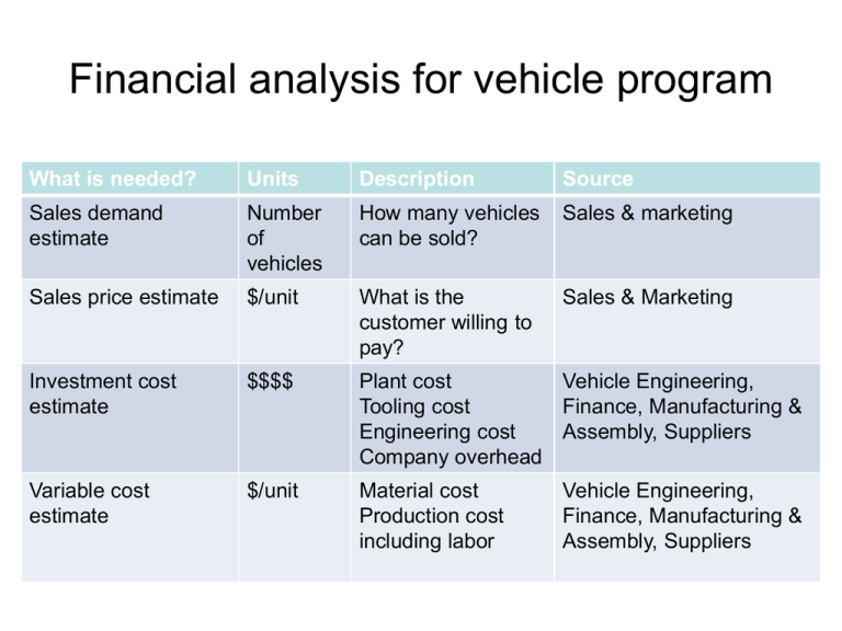
Financial analysis for vehicle program
What is needed?
Units
Description
Source
Sales demand
estimate
Number
of
vehicles
How many vehicles
can be sold?
Sales & marketing
Sales price estimate
$/unit
What is the
customer willing to
pay?
Sales & Marketing
Investment cost
estimate
$$$$
Plant cost
Vehicle Engineering,
Tooling cost
Finance, Manufacturing &
Engineering cost
Assembly, Suppliers
Company overhead
Variable cost
estimate
$/unit
Material cost
Production cost
including labor
Vehicle Engineering,
Finance, Manufacturing &
Assembly, Suppliers
Profit Analysis
Profit = Revenue – cost
Where
Revenue = selling price*number of vehicles sold
Cost
= investment cost + variable cost* number of vehicles produced
Break even volume is the number of vehicles need to be sold so that there is no
loss
Break even Volume = Investment cost/(selling price – variable cost)
Examples of Successful & Unsuccessful
Programs
Entity
Estimate
Actual
Actual
Actual
Sales Volume
150,000
120,000
75,000
150, 000
Sale Price
($/unit)
22,000
22,000
22,000
18,000
Investment
Cost ($)
500 M
500 M
500 M
500 M
Variable Cost
($/unit)
17,000
17,000
17,000
17,000
Total Profit
(M$)
250 M
100 M
- 125 M
-350 M
Break even volume = 500,000,000/(22,000-17,000) = 100,000 vehicles
Your Calculations
1.
2.
3.
4.
5.
6.
Estimate selling price for your car from market survey
Estimate the number of vehicles that can be sold
Assume variable cost to be about X% of the selling price
Assume investment cost to be Y RM
Figure out break even volume and profit
Figure out a way to distribute investment and variable cost to systems
Investment
Cost
Body
Chassis
Powertrain
Climate Control
Electrical
Variable
Cost
Body
Chassis
Powertrain
Climate Control
Electrical
Weight Analysis
Curb Weight : Weight of an assembled vehicle
Gross Vehicle Weight (GVW) = Curb weight + passenger & cargo weight
Corner weight = weight on each suspension
Curb
Weight
Body
Chassis
Powertrain
Climate Control
Electrical
Vehicle-fixed Coordinate System
• ISO (International Standards Organization)
coordinate system
• Defines directions with respect to the vehicle
Z Vertical
Yaw
r
Rol l
p
CG
q
Pitch
X
L
i na
it ud
g
n
o
l
Y
L ate ral
Forces Acting on a Car, Truck or
Motorcycle
h
B
Fx
f
Mg
x
M g
c os

Ma
sin 
Mg
LA
PM
b

d
D
A
F
zf
L
A
L /2
c
R
h
hx
h
h
Fx
r
R
hz
F
zr
•
•
•
•
•
•
Gravity
Moment Equations
Tire
normal forces (loads)
Taking moments about point A
Tire shear forces (driving or braking)
Aerodynamic forces and moments
Taking moments about point B yields
D’Alembert (acceleration) forces
Trailer hitch loads
 M A= FzfL + M a hx+ M g h sin
c
Fzf = M g cos
L
b
Fzr= M g cos
L
L
 - M g c cos
h
h
 - M a x - M g sin
L
L
h
-
h
 + M a x + M g sin
L
L
 + L A + PM + R h hx
+ R h d = hz
0
2
LA
-
-
2
LA
+
2
PM
-R
L
PM
+R
L
h
- Rh
hx
L
hh
+R
hx
L
dh
hz L
dh + L
hz
L
h
Static Loads
• Sitting statically on a level surface:
W fs  M  g c
c
L
W
c
L
W rs  M  g c
b
L
W
b
L
Longitudinal Dynamics
•
•
•
•
Dynamic load transfer
Acceleration limits
Braking limits
Aerodynamic forces/moments
Acceleration at Low Speed
• Acceleration on a level surface with no
aerodynamic reactions
Wf W (
c

L
Wr  W (
h ax
L gc
b
L

)  W fs  W
h ax
L gc
h ax
L gc
)  W rs  W
h ax
L gc
Climbing a Grade
• No aerodynamic or acceleration effects
Wf W (
c  cos 

L
h
sin  )
Wr  W (
b  cos 
L

h
sin  )
L
L
• For small angles: cos = 1, sin = 
W f  W fs  W
h

W r  W rs  W
L
•  = Grade angle (in radians)
h
L

Aerodynamic Resistance Load
Aerodynamic drag load
DA = 0.5 ρ V2 CD A
Where:
CD = Aerodynamic drag Coefficient
ρ
A
= Air density
= Frontal Area of the vehicle
Tire Rolling Resistance Load
Rolling resistance load
Rx = Rxf + Rxr = fr Wf + fr Wr
Where:
fr
= Rolling Resistance Coefficient
Wr
= Rear axle load
Wf
= Front axle load
fr = 0.015 or 0.01*(1+ V/160)
Where, V is vehicle speed in km/h
Powertrain Applications
• Powertrain development
– Architecture evaluation (FWD, RWD, 4WD)
– Acceleration (0-100 kph, passing), top speed
– Tuning (engine, torque converter,
transmission matching)
– Traction limits
– Fuel economy
Powertrain Architecture
• Traction-limited acceleration depends on loads on the
drive wheels
• I.e., F    F
x
z
Front wheel drive
Rear wheel drive
Four wheel drive
Powertrain Architecture
• Components in a solid axle rear drive
Engine Dyno Performance
• Steady speed; Wide Open Throttle (WOT)
Basic Acceleration Model
Fx  M  a x 
a x  Fx
ax
gc

gc
W
=
W
gc
ax
and P  F x  V
P gc
V W
1 P
V W
• Simple acceleration model used by highway engineers
• Acceleration is:
– Proportional to power to weight ratio
– Inversely proportional to speed
Example of Simple Model
• Simple acceleration model used by highway engineers
– It over-predicts performance with actual P/W ratios
– Models are calibrated with effective P/W ratio
1
Simulated Vehicle (250 kw, 1833 kg, with all losses)
0.9
100% Efficient
0.8
Acceleraiton (g)
0.7
50% Efficient
0.6
0.5
0.4
0.3
0.2
0.1
0
0
20
40
60
80
100
Speed (km/h)
120
140
160
180
200
Tractive Force Performance
• Tractive force vs. speed:
– Reflects engine torque
curve
– Depends on gear
• Low (1st) gear
– High tractive effort
– Limited speed range
• Higher gears expand the
speed range but reduce
tractive effort
• Multiple gears approximate constant engine power
• Continuously variable transmission (CVT) can follow constant engine
power curve
Acceleration Performance
(M+Mr) ax = T Ngf ηgf/r – Rx – DA – Rhx – W sinθ
Where
M = vehicle mass = W/g
Mr = equivalent mass of rotating components
ax = longitudinal acceleration
T = Engine Toerque
Ngf = combined ratio of transmission & final drive
ηgf = combined efficiency of transmission & final drive
Rx = Rolling resistance forces
DA = Aerodynamic forces
Rhx = Hitch forces
θ
= Inclination angle
Mr = [(Ie+It)Ngf2 + IdNf2 + Iw]/r2 or Mr/M = 0.04Ngf+0.0025Ngf2
and Ie,It and Iw are engine, transmission, axle inertias
Top Speed Calculation
T Ngf ηgf/r >= Rx + DA + Rhx + W sinθ
If LHS > RHS, acceleration to higher speed is possible
LHS = RHS corresponds to top speed in that gear
Powertrain System Design
Uncontrolled
Variables
Aerodynamic Drag
Rolling Resistance
Climbing Grade
Mass, Driveline Inertias
Gear Inefficiencies
Vehicle
Design Specifications
•Engine torque/power
•Transmission Gear Ratios
•Final Drive Gear Ratio
•Torque Converter
•Tire Size
•Tire Traction Limit
•Axle Roll
Acceleration
Top Speed
What is needed?
• Procedure for calculating top speed and
time to reach 100 km/h from 0
• Procedure to calculate top speed
• spreadsheet
Torque Converter
• Fluid coupling between engine
and transmission
• Stator:
– Deflects return flow in direction of
the impeller
– Adds to torque of impeller
– Turbine torque > engine torque
• Zero output/input speed ratio is
“stall”
• Turbine input to transmission is
typically two times engine
torque
Differential
Differential Rules
R ul es for F ree D iffer entials
Tleft  Tright 
Pinion
Gear
Ring
Gear
 left   right
Carrier
2
Tcarrier
2
  carrier
Axle
Shaft
Axle
Shaft
Side
Gear
R ul es for Lo cking D iff eren ti al
Carrier
Gear
Tleft  Tright  Tcarrier
 left   right   carrier
Torques on a Chassis
Traction Limits
 W
 W
F x m ax 
1 
h

Fx m ax 
b
1 
L
2  r K f
L
N ft
h
F x m ax 
 W
F x m ax 
1 
L
h
L
1 
L
2  r Kr
N ft
K
 W
b

L
c
c
L
h
L
K
Differential Performance
Brake Systems Applications
• Proportioning evaluation
– Weight variations (curb weight to GVWR)
– High and low friction
• Testing for regulatory compliance (FMVSS
105, 121..)
• Stability in braking (e.g., split mu, FMVSS
135)
• Evaluating effect of partial system failures
Typical Braking System
Rear
Brake
Vacuum
Assist
Re a
r
Brake
Pedal
b ra
ke
Master
Cylinder
lin e
s
Parking Brake
Combination
Valve
t
ne
o n e li
r
F ak
br
s
Front
Brake
Tire Slip
Tire

V
Slip (S) =
Vertical
Load
Friction
Force
Relative
Slip
V- r
V
0.8
B ra kin g Co e fficie nt
Contact
Length

p
30 m
0.6
ph
Dry
Adhesion
0.4
30 m

s
ph
We
t
0.2
Hysteresis
0
0
20
40
60
Wheel Slip (%)
80
100
Wheel Lockup
• Front wheel lockup will cause loss of
ability to steer the vehicle
• With rear wheel lockup, any yaw
disturbance will initiate rotation of the
vehicle making it unstable
• Brake proportioning strategy should allow
the front brakes to lock first if ABS is not
provided
Anti-lock Brakes
0.8
1
le S
pe
ed
2
3
0
1
2
3
4
Time (sec)
5
6
7
Cycling
0.6
3
1
c a ti o n
RF
h ic
2
0.4
A p p li
Ve
LF
B rakin g C oe fficie nt
W he el S p ee d
LR
RR
0.2
0
0
20
40
60
Wheel Slip (%)
80
100
FMVSS Regulatory Requirements
1.
2.
3.
4.
A fully loaded passenger car with new brakes will stop from
speeds 30/60 mph in distance with average deceleration of
17/18 ft/s^2
A fully loaded passenger car with burnished brakes will stop
from speeds 30/60/80 mph in distance with average
deceleration of 17/19/18 ft/s^2
A lightly loaded passenger car with burnished brakes will
stop from speeds 60 mph in distance with average
deceleration of 20 ft/s^2
A fully and lightly loaded passenger car with brake failure
will stop from speeds 60 mph in distance with average
deceleration of 8.5 ft/s^2
Brake Proportioning
Maximum brake force an axle can carry without locking
μp(Wfs + Fxr*h/L)
Front Axle Fxmf = ------------------------1 – μp*h/L
μp(Wrs - Fxf*h/L)
Rear Axle Fxmr = ------------------------1 + μp*h/L
Where Fxf and Fxr are front and rear brake forces
Wfs and Wrs are front and rear static weights
μp is the peak brake coefficient
h is the c.g. height
L is the wheelbase
Brake Proportioning
Brake Force Fx = Tb/r = G Pa/r
Where
Fx is front or rear brake force (N)
Tb is front or rear brake torque (Nm)
r is the tire rolling radius (m)
G is front or rear brake gain (N.m/MPa)
Pa is brake application pressure
What is needed
• Explanation on how to draw braking limits
on the chart
• How to draw FMVSS requirement
• How to draw applied brake force diagram
• Brake pressure/brake torque relation
• Brake proportion strategy graph
Performance Triangles
Slope 
 p W fs
1 p
Front Brake Force
2000
p h
L
h
1 p
h
L
Slope 
 p h
L
h
1 p
L
1500
Proportioning
Range
1000
500
 p W rs
1 p
0
0
500
1000
h
L
1500
Rear Brake Force
2000
L
Brake Proportioning
1st Effectiveness
F ro n t B ra ke Fo rce (lb)
2000
2nd Effectiveness
3rd Effectiveness
1500

= 0.3, lightly loaded

= 0.3, GVW R
1000
Proportioning
Line
500
500
1000
1500
Rear Brake Force (lb)
2000
Braking Efficiency
Eb = Dx/μp
Where
Eb is the braking efficiency
Dx is the actual deceleration
μp is the braking coefficient
Braking Efficiency Calculation
1. Assume front and rear brake proportioning strategy such as
Pf = Pa and Pr = 0.8 Pa
2. Calculate front and rear axle brake forces
Fxf = 2Gf*Pf/r and Fxr = 2Gr*Pr/r
3. Calculate deceleration Dx
Dx = (Fxf+Fxr)/W
4. Calculate front and rear axle loads
5. Wf = Wfs + (h/L)(W/g)Dx
Wr = Wrs – (h/L)(W/g)Dx
5. Calculate braking coefficients μf and μr
μf = Fxf/Wf and μr = Fxr/Wr
6. Calculate braking efficiency Eb
Eb = Dx/ (higher of μf or μr)
7. Increase Pa till desired level of Dx is reached
Brake System Design
Uncontrolled
Variables
Aerodynamic Drag
Rolling Resistance
Mass, C.G., wheelbase
Vehicle
•Brake Pressure
•Brake Torque Gains
•Brake Proportioning
•Tire Size
•Tire Friction Limit
Design Specifications
Deceleration
Efficiency
Locking Strategy
Energy/Power Absorption
Energy and power absorbed by the brake system during braking
E = MV2/2
P = MV2/(2ts)
Where
M is the mass of the vehicle
V is the initial speed
ts is the time to stop