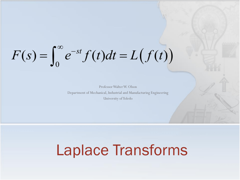
 
0
  e st
( )
 
( )

Professor Walter W. Olson
Department of Mechanical, Industrial and Manufacturing Engineering
University of Toledo






Review





Phase
Phase Computations
Full Bode Plot
System Identification
Using Bode Plots for System Identification
Laplace Transform
Inverse Laplace Transform
Properties of the Laplace Transform
Final Value Theorem

 s
 i
 
( )
 e
 cos
   i sin
 

( )

(

) e

Me
 i
   t where M

(

) is the magnitude or gain of
 
and tan

1


Im
Re


 
 




is the phase angle or argument of
 


For a sinusoidal input, phase represents the lag of the system or, alternatively, the processing time of the system to produce an output from the input
Phase is measured as an angle


A cycle of the input is consider to take 2 p radians or 360 degrees
Phase is the angular distance it takes for the output to represent the input


Thus it is normal that as the frequency increases that the phase also increase
In the case where the phase exceeds 180 degrees, the output appears to
“lead” the input. This is particularly evident in the range of 270 to 360 degrees.


G s tan

1


Im
Re


 
 






As with magnitude there are 4 factors to consider which can be added together for the total phase angle.
We will consider, in turn,

K
 s n
  a )

( s
2 
2
 n s
  n
2
)
 The sign will be positive if the factor is in the numerator and negative if the factor is in the denominator


K is the angle of a real number; therefore it is always 0 (or 180 if the number were negative) n
( i
 n
) n
for n
2 i 180
 the angle of complete turns (n )
for n
2 i
 
0

the angle of complete turns (n )
If n is an o i
 i i
for
for n n

1
2

1
an ev i i 270

the angle of complete turns (n )
2 i i : s 90

the angle of complete turns (n )
Examples: s 90
 s

1
1 s
90
 s

2 
-180
 s

3
= -270
 s

5  
90

360
 
450

( s a )
 
( i
  a )
 arctan
Where

Where
 a
Where
10 a , arctan a , arctan
 a
 a
0
90
0 a
Where
10
 a line from 0 to 90

( s
2 
2
 n s
  n
2
)
 
(

 n
2  
2

 i 2
  n
)
 arctan 


2
 

2
 n
 2
This now also involves the variable,




Where
  n
, arctan
Where
  n
, arctan
 a
 a
0
180
0
 a line from 0 to 180 with a correction for


sys




It is not unusual for a field engineer to be shown a piece of equipment and then asked if he can put a control system on it or replace the control system for which there are no parts.
The task of determining how an unknown structure responds is called “System Identification”.
To identify a system, there are many tools are your disposal




First and foremost, what should the system structure look like?
 Motors are often first order transfer functions ( ) which you then attempt to identify the constants s
K
 a
Perform step tests and see what the response looks like
Perform tests with sinusoidal outputs and use the Bode plot to identify the system
Apply statistical/time series methods such as ARMAX and RELS







The overall order of the system will be the high frequency phase divided by 90 degrees
The exponent of the “s” term will be the slope on the magnitude plot at the lowest frequency divided by 20
 Alternatively, the exponent of “s” is the lowest frequency phase divided by 90 degrees.
The system gain constant (K t
) in dB will be the height value at the extension of the “s” term line on the magnitude plot to where it crosses1 rps
Starting from the left (the lowest frequency) on the magnitude plot, determine the structural components using the change in slopes in increments of 20 degrees either up or down
Then by using the intersection of the lines at those places match to the test curve, determine the break frequencies
Write the transfer function in the form
( )

K t s p



 s b
1 s a
1

1



1
 b s
2 s a
2



1 ...

 

1 ...



  s b m a s q


1

1

 s
2
 nz s
2
1
2
 np 1
2


2


2 nz 1

 z 1 s p 1 np 1 s


1



1


 s nz

2 s
2 np
2
2
2
2


2

 nz
2
2 s
2
 p 2
 np 2


1 ...
s


1 ...





Traditionally, Feedback Control Theory was initiated by using the Laplace Transform of the differential equations to develop the Transfer Function
The was one caveat: the initial conditions were assumed to be zero.
 For most systems a simple coordinate change could effect this
 If not, then a more complicated form using the derivative property of Laplace transforms had to be used which could lead to intractable forms
While we derived the transfer function, G(s), using the convolution equation and the state space relationships, the transfer function so derived is a Laplace Transform under zero initial conditions



CAUTION: Some Mathematics is necessary!
The Laplace transform is defined as
(i.e., integrable everywhere and everywhere less than e s
0
 
0
  e st
( )
 
( )
 s is a complex number
The Inverse Laplace transform is defined as

1
2 p i
 st
( )

L

1

( )

Fortunately, we rarely have to use these integrals as there are other methods

Tables are available for determining the Laplace transform of most common functions
This table which continues on the next slide is from Modern Control
Engineering by K. Ogata
4 th ed., 2002

 
0
  e st
( )
 
( )

 Note that the index on the integral is 0:
 it is assumed that no dynamics are considered prior to t=0
( )

0 t

0
 The Laplace is a linear transform:
( ( ))
 
0

 st
( )
 a

0
 e
 st
( )

   
      
 
0
  e st
       dt



0


 st
 
  




0

  
 st
 




The Laplace Transform of the
Impulse Function

L
 

( )







1

0 t

0
0
 t<

0 t

0
1
The Laplace Transform of the
Step Function


0 t<0
1 t

0
L
 

1 s
The Laplace Transform of a
Unit Ramp:
0 t<0
 t t

0

1 s
2


The Laplace Transform of the
2 nd power of t:
0 t<0
 t
2
2
t

0

1 s
3
The Place Transform of the n th power of t:
0 t<0 t n
 n !
t

0

1 s n

1

 Laplace Trans Form of the exponentials:
0 t<0
 e
 at
t

0

1 s
 a
 Laplace Transforms of trigonometric functions:
0 t<0 sin
 t t

0
 s
2

 
2
0 t<0
 te
 at
t

0

1
 s
 a

2
0 t<0
 t e
 at
t

0
 n !
 s
 a
 n

1
0 t<0 cos
 t t

0
 s
2 s
 
2

 e
 at

0 t<0 sin
 t t

0

 s
 a

2  
2

 Find the Laplace Transform of f t
  
17
   


2
4 t 17
 
L
  
L
 
 

L
  
L
   s
2
3
 s
4
2

17 s
 Find the Laplace Transform of ( )

4 sin(3 t

2)
Notice that this one has a phase (2) and there are no transforms in the tables for this

( )

4 sin(3 t

2)

     
( )
 
L

4
 s
      


 
L
   
  
L
   

( )
    s
2
3

9

4 sin(2) s
2 s

9 and then evaluate the constants
  
3.6372
s

4.9938
s
2 
9

Find the transfer function for this system with voltage as the input and angular position as the output using Laplace Transforms








Voltage Loop: R i a a

V b

V a
Back Voltage: V
Rotations NSL: J b d

K
Motor Torque: T

Ki a
2 dt
 b
 d b
 dt d
 dt i a
K d


V
R dt R a a


 d 2
 dt

Ki a
 b d

J J dt

T d
2
 dt


 s 2

 b
J

KK
JR a b

 d
 dt

KV
JR a a


 b
J

KK
J R a b

 s




( )

KV a
 
JR a

K
( )

V
 a
 
 s 2
JR a


 b

KK
J JR a b

 s
V
 a
 

JR s a
2
 
K bR a

KK b
 s

L

1

1 s
 a  e
 at
L

1



1 s s
 a


 
1 a

1
 e
 at

L

1


 s
 a
1
 s
 b


  b
1
 a
 e
 at  e
 bt

L

1

 s
2 
 n
2
2
  n
 n
2



 n
1
 
2 e
 i
 n t sin

 n t 1
 
2


 Find the Inverse Laplace Transform of
L

1

( )
 
L

1
10 s
2
 s

10 L

1



1

1


 

 e
 t


10 s
2  s
 Find the Inverse Laplace Transform of  s
4
300

36 s
2
L

1

( )
 
L

1 s
4
300

36 s
2

300 L

1

 s
2
 s
2
1

36



L

1

( )
 
300
216
L

1

 s
2
 s
2
6
3

6
2


 
L

1

( )
 
8.3333
t
  
300
216

6 t
   

 Laplace Transforms have several very import properties which are useful in Controls
L d dt
( )
 

( )
 f (0)
L

 d dt
2 f t


 2
( )
 sf (0)
 d dt
L


0 t f t dt

 s f (0)
Now, you should see the advantage of having zero initial conditions

 If f(t) and its derivative satisfy the conditions for Laplace
Transforms, then t
 f t
 s lim

0 sF s


This theorem is very useful in determining the steady state gain of a stable system transfer function
Do not apply this to an unstable system as the wrong conclusions will be reached!

 What is the steady state gain (DC Gain) of the system

3
 s

2


2 
2 s

10
 t
 g t
 s lim

0 sG s
 s lim

0
3
 
2


2 
2 s

10


0.6





Laplace Transform
Inverse Laplace Transform
Properties of the Laplace Transform
Final Value Theorem
Next Class: Using the Laplace Transform