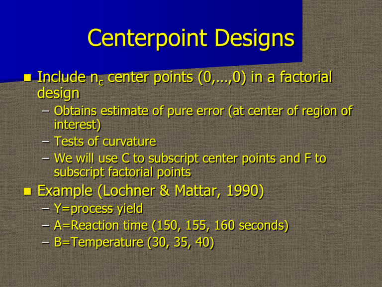
Centerpoint Designs

Include nc center points (0,…,0) in a factorial
design
– Obtains estimate of pure error (at center of region of
interest)
– Tests of curvature
– We will use C to subscript center points and F to
subscript factorial points

Example (Lochner & Mattar, 1990)
– Y=process yield
– A=Reaction time (150, 155, 160 seconds)
– B=Temperature (30, 35, 40)
Centerpoint Designs
+1
B
41.5
40
40.3
40.5
40.7
40.2
40.6
0
-1
39.3
-1
40.9
0
A
+1
Centerpoint Designs

Statistics used for test of curvature
yC  (40.3  40.5  40.7  40.2  40.6) / 5  40.46
yF  (39.3  40.9  40  41.5) / 4  40.425
sC  .20736
Centerpoint Designs
When do we have curvature?
 For a main effects or interaction model,

yc  yF

Otherwise, for many types of curvature,
yc  yF
Centerpoint Designs
•A test statistic for curvature
yC  yF
T
1
1
sC

nC nF
Centerpoint Designs
T has a t distribution with nC-1 df
(t.975,4=2.776)
 T>0 indicates a hilltop or ridge
 T<0 indicates a valley

40.46  40.425 .035
T

 .25
1 1 .139
.20736 
5 4
Centerpoint Designs
We can use sC to construct t tests (with
nC-1 df ) for the factor effects as well
 E.g., To test H0: effect A = 0
the test statistic would be:

T
A
sC
2
k 2
Follow-up Designs
If curvature is significant, and indicates
that the design is centered (or near) an
optimum response, we can augment the
design to learn more about the shape of
the response surface
 Response Surface Design and Methods

Follow-up Designs
If curvature is not significant, or indicates
that the design is not near an optimum
response, we can search for the optimum
response
 Steepest Ascent (if maximizing the
response is the goal) is a straightforward
approach to optimizing the response

Steepest Ascent
The steepest ascent direction is derived
from the additive model for an experiment
expressed in either coded or uncoded units.
 Helicopter II Example (Minitab Project)

– Rotor Length (7 cm, 12 cm)
– Rotor Width (3 cm, 5 cm)
– 5 centerpoints (9.5 cm, 4 cm)
Steepest Ascent

Helicopter II Example:
RL * 9.5
RL 
 RL*  9.5  2.5 RL
2 .5
RW * 4
RW 
 RW *  4  RW
1
Steepest Ascent

The coefficients from either the coded or uncoded
additive model define the steepest ascent vector
(b1 b2)’.

Helicopter II Example
2.775+.425RL-.175RW=
2.775+.425(RL*-9.5)/2.5-.175(RW*-3)=
(2.775-1.615+.525) + .17RL* -.175RW*=
1.685+.17RL*-.175RW*
Contour Plot of Flight Time (Seconds) vs Rotor Width, Rotor Length
5.0
2.8
2.4
RotorWidth
4.5
4.0
3.2
3.5
2.6
3.0
7
3.0
8
9
10
RotorLength
11
12
Steepest Ascent
With a steepest ascent direction in
hand, we select design points, starting
from the centerpoint along this path and
continue until the response stops
improving.
 If the first step results in poorer
performance, then it may be necessary
to backtrack
 For the helicopter example, let’s use (1,
-1)’ as an ascent vector.

Steepest Ascent

Helicopter II
Example:
Run
RW*
RL*
1
3
12
2
2.5
12.5
3
2
13
4
1.5
13.5
5
1
14
Steepest Ascent




The point along the steepest ascent direction
with highest mean response will serve as the
centerpoint of the new design
Choose new factor levels (guidelines here are
vague)
Confirm that yC  yF
Add axial points to the design to fully
characterize the shape of the response surface
and predict the maximum.
Central Composite Design
1.5
Block s
1
2
1.0
X2
0.5
(0,0) includes 3 Block 1 runs
and 3 Block 2 runs
0.0
-0.5
-1.0
-1.5
-1.5
-1.0
-0.5
0.0
X1
0.5
1.0
1.5
Steepest Ascent


The axial points are chosen so that the response at
each combination of factor levels is estimated with
approximately the same precision.
With 9 distinct design points, we can comfortably
estimate a full quadratic response surface
E(Y | X )  b0  b1x1  b2 x2  b11 x12  b22 x22  b12 x1x2

We usually translate and rotate X1 and X2 to
characterize the response surface (canonical
analysis)