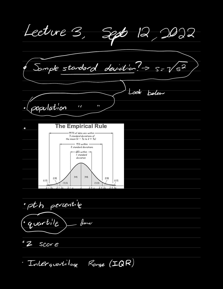
Lecture
3
Sept 12,2022
Samplestanda
zU
ddah.in
Population
a
pth percentile
aquartile
c
z
doo
score
Interquartilage
Range
IOR
os
Look
been
q
ge.gg
C
Box plots
example calculate variance for
n
5
2
8
1320
EBI.IE
s
13201281
80
x
1320gEE
10
standard deviation
is
can
shown
originalunits
in
be
an
M 26 M
x
25
I
E
S
M
E
MTG
E
S
ME
I
2s
Example
217.5
0
IFL
38
Er
which
510
Me
are
100
To
48
70
15
5
80,105
50
outliers
2
2
3.336
59511
2280501
2
105,5100 20.33
CHAPTER
Sample
1.33
Point
3
X
X
PROBABILITY
Basic outcome
of
expirement
p
Lecture
4
1512022
Sept
Color Number
1000
25
Red
Total 100
Brown 20
probability of yellow
Find
20
Green
15
Blue
Yellow
10
Orange
10
Ide
28
es
diet
died
3
51
I
20
chance
yellow
1
or
or
74
a
orange
of getting
orange
Tsao
of
Multiplaciative role
Prob distribution of
random
a
probability
discrete
variaby
Bayes Rule
Eg From YT
A
1.2
P
j 7
3,45
I
PIBIA
occurs
has
13
Probability that
given that
already occurred
4,5 6,7 8,9
A
B
PCA B
3
B
A
I 8
13
PCA
PCB
Eg
Eg
5
PIBIA
B
given
12,3 4.5 6.7
8,9
under
only 2 fall
that A has
occurred
data
points
PBÉÉ
pears
24ft
9
2
6
1
3
CHECK ANSWER
PAGE
PGY8
PCB
3
8
IT
82
Prof
From YT
0.12
cl
PRAFPHIjfg
PH
0.9nd PCt
O 06
4
0841
Pratt
Tor
PINCH
Nc
C
0.68345
In
Pf
t
Pfe and
0.95
60,12
PCNC and
C
88
0.1668
Visualmethed
yooo
t1
0.061
t
100
T
10000
760
880075180
8272
Plot
wi
18
so
0.60
Probability
of
intersection
Independent events
Lecture6
Sept22_
Mean of
a
Variance
discrete random
of random variable
Binomial random variable
WTF
variable
of 2
Cumulative
Binomial
in
Poisson
distribution
Distribution
0.577
0.577
function
Probabilities
Look
ex on
235
240
what is g
q
Do
Erik
Fun
Chapter
6
Sampling
Oct 6
18 tan
5
Édndom
sample
EFI
E
M
6.1 Population is
E
6.2
CLT
NIM
n
normal
Er
730
6
E
Distributions
ENN
M
En
Sampling
7
Chapter
on
the
of
Distribution
sample proportion
based
Inferences
single sample
a
Where
find
to
confidence
p 282
Confidence coefficient
Oct
13
Review
Practice questions
Confidence
Interval
Download
lecture
11
Standard normal
T distribution
How to use
5
n
t
df
4
If
e
n
2
2
distribution
table
table isn't used
bottom
row
of
t table
can
be used
Sampling distribution
P.M
14115,16
not
ng
p
of
success
of failure
notes thugs
Practice q
Binomial
of
to
learn
1718,19
Poisson
Oct
lecture 15
27
Independent sampling
Sampling
distribution
of
F
52
Test of Hypothesis
1,2
tailed
test
Large sample inferences
Conduct the test
tho M Ma
Pooled estimate to find test
0 against Ha Mi Mato
statistic
Idf
Not
Comparing 2 population Proportions
Properties of the sampling distribution of
es
fp p
452,453,457
How to determine sample size
P value Probability
statistical
that
a
particular
of an
assumed probability distribution will be
greater than
smaller
measure
or
p value
equal to
means
Mio
observed results
more
significant
simpler the probability that random
chance generated the data
or
something else that is equal
or
rarer
No slides posted
2
NYj.vÉ
Chi Square distribution x2
Sum of squares of independent standard
normal random variables 4 2 23 Z
has degrees
sample
sum
I
of
n
of freedom
if
independent squares
normal random variables
venial
n
it
is the
of standard
ri
Conditions required for
a
valid
Large Sample Hypothesis test for
l A random sample is selected from
the target
population
2 The population
selected has
o
a
from which the sample is
distribution that is
approximately
normal
Xp
normal random variable
Xi X2 Xn
Mo
I
z
x
É
1,72
x
T
statistic
unknown
cannot involve parameter
Chi square density
has
asis
If
x
the
is
curve
long
23 Effn
E
I
Var Zi
2n
Z
Z
Elz
EG
right tail right send
var
23 23
8
not symmetric
E
zig
Era
t
n
Var 2,21 2
If
Chi
ga
the
square
conditions
distribution
are
then
satisfied
with
df
n
i
sample variance
nf
tf
n
follows
X
population variance
if
s
then
Hypothesis test
for
is much larger than 62
we have good evidence
population variance 02
62 6.2 Ha o
Test statistic Zfest
Ho
6
1
02
Ha 02608
n
Z
Ha
6
if Ho is true
too I
x
to rejection region is
d
Mf
for upper tail
PM
x
x
test
N'test
for lower tail test
off
PKC
Test
Ice
Engg
2min
Ex
I
ttk
PLACE D
table only gives
of remaining
for two tailed
Upper
PA Test
upper
tail
g.sn
tail
area
test
z2jz2q
22
for lower tail
Rejection region
has df
find
n
area
l
Ex A
random sample
n
selected
observations
the Ho
test
used to
is
population
the
of
from a normal
52 155 Specify
appropriate rejection region
Ha 027155
25
n
0.10
0
uppertailed
test
I
Mfs
24
8.2 Lab A
Lab B
a
Try
na
test
to
b
Test
a
Lab A
8
19
N
3.3.1963
5.56
6.36
51
6.35 52 6.03
whether lab A has variance greater than 6
I2
20
Lab B have equal
whether LabA
variance
so
variance
22 distribution
use
Let
0
6
0
0.05
0.05
denote variance
of LabA
Ho 6.2 6
test
v3
95
Ha
statistic
1
42
6
O
19
0838
den
1
check Z
rejection region is
Tests28.869
20.2248
not
7277218.005
in 95
18
table
28.869
rejection region thus do not
confidence
reject Ho with 95
p value PA 720.24481 is between
0.9 and 0.1
It
1
d
greater than
Nov 15,2022
F distribution
o.o
Do
n
d 0.1
reject Ho with 45
not
Ratio of two
distributions
independent
of
freedom
1
The 2 populations
2
The samples
are
selected from their
I
O
No notes posted
Has degrees
Conditions
be
1
is
I
square
na
normally distributed
independently
respective populations
mz
v
Fn i
n
randomly
n
sÉÉ
are
chi
na
z
1
test for
Hypothesis
2 population variances
Alwaysassumenull hypothesis is true
Ho
Ha 0.20.2
0.2 63
n
f
10011
d
F
n
Fn
ins
IS
statistic
Sa's
1s
i n
1
if 52275
to rejection region
gff.x.gg
Fest
FE
I Mt
I
E
Hair
o
Ee.ES Fn
g anFn
Test
Ha O
Fae 0.05
x
pp feed
o
im
Fest
Fn
fFest
3
in
Fo
4
Pff
Fest
D
value
PIECE
2PfF
PIF
Fest
Fest
i
121
program 2
test
to
determine
the two programs
Ho 0,2
Test
259.1
differ
62
statistic
Ha
f
the variances
if
Use
O
0
0.05
02
3,3 38
17
This test require
in the upper tail
720,120
The rejection
of
1.284
7
0
22
of Fna
inn
From table Foos
region
is
F
1.43
0.025
i
1.43
Since the observed value of the
not
fall
6
63
statistic
test
does
Ho
F 1.284 71.43
rejection region
cannot be rejected There is insufficient evidence to indicate
in the
How to
If
we
j
1
NIN
Denote
0.05
F distribution
use
of
means
0
at
than
more
have
2
that
mean
n
t
X2
X2
Xan
Is
a
Xz
432
Xan
53
3
Xian
Ik
K Xie
the
n
Xia
SSE
of
É
Mr
total sample size
of all samples
Sum of
square
population
X
d
Sample
compare
populations
data
Sample 2
Sample 3
to
by
differences
Xi
It
Énf
within
Fit
groups
SSE
a
sum
of
square
from
Nov 17
To test
2022
No slides posted
Ho M Ma
Ha at least
Conditions
i
2
groups have different
I
Is it
na
samples
selected in
independent
M
Ma
k
i
r
mean
Nh
na ng
k
an
giggyi ÉY
manner
From the le treatment
populations
II
SSE
have distributions
that
Eif
Xi
t
den k
are approximately degrees offreedom
normal
3 The k population
variances
are
equal
6,2 622
8
Sum of
sst
22
saffron
squares
I
I
of
differences within groups
1E.fi
niff 1
I
def
sumofsq.ae
55
5
E EfXij
F
SSE
E Ei Xi EET
Il
SST
E
Xi
I
fi Mt
If
I
2 Xi
Test
FI SSE
Fi Fi
xij 51
0
statistic
Fte
Sst
E
Ii
2
SE
Éf
Musset
Festfollows
E Mst
El
Fir i
n
under Ho
if
E na
At
Ma
Al Me
matte
When testing
significance level d
The rejection region
P value
Ny
is
any
Fest
treatment
group
f
is
probability
Fo
Pff Fest
pygmy
If
SS
K l
SST
error
N
K
SSE
total
n
I
SSI's
MS
Must
Mst
Mst
F
EE
d
PE masse
Which
of
the
requirement for
following
ANOVA
valid
a
is
not
condition
a
F test
for
a
randomized experiment
completely
A The sampled populations all have distributions
which are approximately normal
B The sample chosen from each
sufficiently
C
The
large
variances
of
is
the populations
of
X
all the sample populations
are
equal
D The samples
independent
an
are
chosen from each population
in
manner
Example
A partially completed ANOVA table for
completely randomized
source
SST
Sse
55
Time
7
design is shown here
of
SS
13 11 2
252
Err
11
Total
13
a
II
86422615.3 Ms.EE
86.4
F
Ms
25
12.6 Must
97 5.56
2.2
b How
many treatments
are
involved in the experiment
K 1 2 0
c
Does the data
among
3
provide sufficient evidence
the population
means
Test using 0
No
7
Fail
Ng
2.26
a as
to indicate
difference
a
0.05
is
less than
3 98
with
dF 2
11
Fo
É
N
5.98
o
S
identical
or
F
2
or
O
Independent
P
K
P
P
Pa
Pz
Pk
Nov 22
2022
Test the proportions of more than two outcomes
Binomial experiment has only 2 outcomes S or F I
b Lp q
Multinomial experiment has
education level of
NHL
more
are
le
total
We write
as
P Pa
P Pa
n
of trials is n
Xn MN In
like the highest
5 categories
are
for the multinomial
outcomes
O
some college undergraduate graduate
proportion of each category is denoted
P t Pat in the
outcomes
there
players
Some high school high school diploma
Suppose there
than 2
or
Pal or XnMN
na
n
the
variable x
Pk
n
while
P Pa Prod
Test Formultinomial probabilities
Ho P Pio Pa
Test statistic
where ni
test
is the
n n that
Pao
P
Pro
Ha at leastonestatement in Ho is not true
Mft
of observations
Z
that fall into the ith
the
and
off
Ei's
cell counts
in
When testing at
is 22,723
IN Pio
category
significance
P value
is
are
the egg
under Ho
level
PA
o
rejection region
test
The observations
Conditions
multinomial
are a random
sample
from thepopulation
experiment
giaffinomifferimentwitheadisandroprodoedth
the data
cell
I
2
3
4
total
n
65
69
80
go
300
Does this data
the
using
cell
n
E
the
n
pi
P
Ho
0
12
0.2
1 65
300 0.2
Py
3
4
total
69
so
a
300
30
300 03
0.2
90
16581
300g
81
169
contradict
Test
0.3
Pit Pio
2
60
lnig.fi
0.3
13
0.2
Ha at least I
0.05
I
sufficient evidence to
provide
y y
180,11
1
21
3.05
Ifk
1 3
t.as.w.ae
III
There is not
proportions
sufficient aiden
that the cell
differfrom those given in
Ho
One
multinomial variable
If there
two multinomial
are
can
called
also be
variables
one
way table
it is called Two way table
or
contingency
tab
Variable A
A
Level
B
As
N
A
Are
row sum
Rin
hire
i i
is
is
B2 na
n 22
n23
Mak
R2
Rafn
p
p
n
n
n
Rk
Ran
dumdum
C
C
C
Ca
n total
Pa
Gin
Corn
Crn
É
Variable
A
has S
For
a
Corn
has k
is multinomial
outcomes
and B
is also multinomial
outcomes
total
and B
sample
outcome
j
size
A B
Test statistic
count how many
denote
To test whether 2
Ho Variables
n
as
variables are
are
outcome i
ni
independent
independent
Ha they are
23 14,1 mg
É
traits has A
Ei
dependent
Mid
FpfIIIjp
hasdffK
iunderI
where
Entries.is
ilfs
2
Significance level d
P value
is
Conditions
P X2
N'test
observations
n
Nevis o
rejection region is
are
sample from
random
a
the population
RS
1
Each
Es
outcome
Eiggeted
Do boys and girls
Use
perform differently
midterm
0.05
0
760
460
girls
s
4
17
are
boys
18
11
29
Ha They are
31
15
46
Ei
on
IF
Ho is gender and
hit 13
15,2 4
midterm
performance
independent
É
É
na 18 Ea
E22
22 11
Nov 24
2022
Yes
I.MEiImii ItM
dependent
7,83 11.46
17
2
5.54
1
19.54
281
9.46
o
1.040717
N
From table
II
3 841
a
0
0.05 rejection region is
Thus do not reject Ho
is independent of midterm
0
82783.05 3.841
i.e
0 05
Ho gender
performance
topic
new
µ
I
mean
10 000
1000
2000
More
Maooo
Mio ooo
10
10
10
sale price
90000
150
30000
60 square feet
1000
000
2000
3000
210 000
Real sale price
Y
700
30000 t
60 square feet t
Bo
B
X
E
E
End
Linear regression
yr
yr
i
i
linear
positive
s
trend
If
use
the scatter plot shows linear trend
the simple linear regression model
t
B Xi
Ei
to describe the relation
X
linear
trend
trend
Yi Po
Y
No
Negative linear
of
2
called dependent variable or
is called independent variable or
random
error
component
Bo is the intersect of the
line
B
line
is the slope of
the
on
1,2
X and Y where
is
E is called
could
we
response
variable
predictor variable
BoxBY
ya
BY
ax
Bo
D8
O
Be Ex
and
How to estimate Bo
Use least
SSE
square
sum
B 5s
The line Y
ez
normal
Minimize
SSE
for Bo
denoted
B
to obtain estimates
as
Bo
B
Least
É
ÉÉÉ
BE
Bo Y
line
IIIT
SSE
Denote
of squares of the errors
dqp.to
Iggy
Where
B
B Bix
Yi Yi
is
is called
the
error
least
squares
Properties
1 The
of
sum
the
errors
equal OF
exo
Bist
EY Npo
Y
2 The
B Brito
of squared
sum
errors
for any other straight
line
Sst
is
smaller than that
model
administrators performance
Example
4
14 ooo
pay raise
y
estimated slope
interpret the
Ans For
B
B
a
yooo
of
the
line
2 point increase in an administrators rating we
estimate the administrators raise to decrease by 2000
a
M
Assumptions of linear
regression
1 Mean
of
error
E is o
2 Variance of E is
3 E is normal
4 Ei
Is ish
are
a
s
constant 02
independent
s
EC
Yl
SEE
Nov 29
2022
2
yEYM_s
µ
estimation of 02
52 5121
SSE
g pipe
II
estimation of
S
Fa
Ely Bo Bxd
standard da
SEF
we
o
of
refer to
standard
error
E
we
s
as
use
the
estimated
of the regression model
Interpretation of S
expect most f 95 1 of the observed values to lie
within 2s
least squares predicted values
of their respective
we
To test
Ha
B
B
i.e
o
Ho
B
0
Ha
B
Ha B
0
I
whether X Y
linear
O
has
p
Whether
8,4 has
positive linear
relation
relation
B
B
will be normal with
I
É
e
Gp by
estimate
the
estimated standard
z
of
FEELS
negative
linear
N 0,02
the sampling dist
and standard deviation
9 555
and refer
B
B
hypotheggedvaluetffs
SE
XY has
E
Spiff
error
B
mean
o
we
whether
relation
Sampling distribution of
If we make the U assumptions about E
of
o
Effi
Ég
E
a
Xi na
ki
to
Sp
as
teese
confidence
10011 07
level
significance
Ha
Iti
B
is
ta Sp
I
rejection region is
a
o
Ha
to
t
B
B
interval for
B
Ha
0
If
to
Plt test
2pct Ittest
o
tot
tot
P value
B
Pftest
may be
Esample
final
on
the number
Is
in
a
of
Data from 14
teams
statistics
summary
8
XI 3.642
Assume
were
major league baseball team
a
collected
and the
yield
2
0.948622
455.27 and 5 9.18
B
by
the teams batting average
related to
season
won
games
Conduct
a
8 85
test to
2
determine
if
a
positive linear relationship exists between
batting average
Ho
B
0
Ha
and number of wins
B
0
I
Use
0
0.05
team
Big
and
55
4553,331 1.704
5
Cfto oona
0.248622
Since the observed value of the
test statistic does not fall in the
Ayy
f
rejection region
1.7047 1.782
Ho cannot be rejected
insufficient evidence to
team
wins
is
There is
indicate that
positively linearly
related to team batting average
Correlation coefficient
É
i
is measure
of
the strength
relationship between 2 variables
of
the linear
8
and
g
tried
if
if
if
ryo
no
r 0
r
there
there
is
is
regather
no
I
crime
rate
casino employee
ted
relation between
linear relation between
allpathos locate in the
if rel
if
there is positive relation between Sand Y
S
line
regression
f
Y
Y
Dec
2.2022_
Last
Class
Er to review correlation coefficient
A low value of the correlation coefficient
X and Y are unrelated
Y
B False
A True
y
y
r
implies that
iI
JESS
BotB.xtgq.ly
E
will be low
Bgt
but there is
fy JESSE correlation
r
I
obviously
a
g BotB x
SSE CSS
ss
Coefficient of determination
Ra
ra
55935,555
1
555
the
total sample variability
represents the proportion of
around y that is explained
by the linear relationship between
It
P
y
Y and X
Interpretation 100
by the total sum
of
ra
the sample variation in y
of
of squares
measured
of the
the deviations
can
be explained by
sample y values about their mean j
in the straight line model
using s to predict
y
In
simple linear regression
coefficient
BotBix y
y
B Bx
is the square
r
of correlation
1 The standard deviation of
the sampling distribution of
the estimator of the mean
y
value of y at a specific
value of X say
Xp is
i
Xp
7
55014 85
refer
we
error
2 The standard dotation
the predictor
Gy
g
y
of
of
an
of
Gg
as
the standard
y
the prediction
individual
fittnI
to
new
we
error
at
y value
refer to
the standard
prediction
for
Xp is
org g
error
of
as
B Bix g
Var ypg
S
100
is
IFI
l d
To
of Y
confidence
interval for
t.IT
02
Gy
mean
prediction interval for
at
X
Xp
an
Y at Exp
individual
new
value
is
X outside the sample range
É
FIjj
We should not make estimation
errors
value of
IgF
t.FI
large
Var y
o
Y
10011 d
Vary
of
of
predictionForvalues
X which
can
lead to
of
Er
9
A
2700
202
n
company's sales
Bo
revenue
banks
charges
Interpolate the estimate
of
Bo
of the line
Answer There
a
sales
is
the y
intercept
practical interpretation since
no
revenue
of
0 is
a
nonsensical value
Ex 2 The least
squares model provides very good
estimates of y for values of X far outside the
contained in the sample
range of x
A True
B False
I
Don't estimate outside
range of X