Using Your TI-83/84/89 Calculator: Linear Correlation and Regression
Dr. Laura Schultz
Statistics I
This handout describes how to use your calculator for various linear correlation and regression
applications. For illustration purposes, we will work with a data set consisting of the Amazon.com
prices of ten commonly adopted introductory statistics textbooks (in $) paired with the page count
for each textbook. You can find this data set in the Appendix at the end of this handout.
1. Before we can get started, you will need to enter the textbook data into your calculator. We will
be using this data set for several different applications, so it will be helpful to enter the data into
named lists. Press Se. Insert a list by highlighting L1 and
pressing `d. Name this list PAGES and proceed to enter the page
count data into this list. Insert another list named PRICE and enter the
Amazon.com prices into this list. Check over your lists to make sure
you didn’t enter any incorrect data values. Note that each PAGES value
must be paired with the corresponding PRICE for a given textbook.
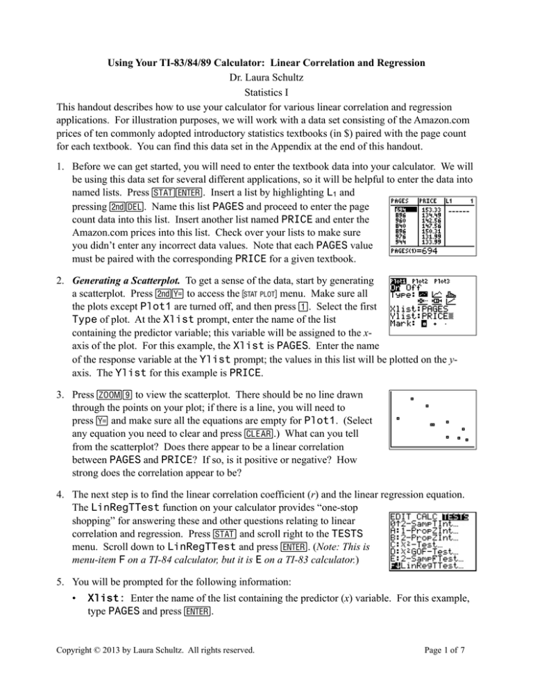
2. Generating a Scatterplot. To get a sense of the data, start by generating
a scatterplot. Press `! to access the , menu. Make sure all
the plots except Plot1 are turned off, and then press 1. Select the first
Type of plot. At the Xlist prompt, enter the name of the list
containing the predictor variable; this variable will be assigned to the xaxis of the plot. For this example, the Xlist is PAGES. Enter the name
of the response variable at the Ylist prompt; the values in this list will be plotted on the yaxis. The Ylist for this example is PRICE.
3. Press #9 to view the scatterplot. There should be no line drawn
through the points on your plot; if there is a line, you will need to
press ! and make sure all the equations are empty for Plot1. (Select
any equation you need to clear and press C.) What can you tell
from the scatterplot? Does there appear to be a linear correlation
between PAGES and PRICE? If so, is it positive or negative? How
strong does the correlation appear to be?
4. The next step is to find the linear correlation coefficient (r) and the linear regression equation.
The LinRegTTest function on your calculator provides “one-stop
shopping” for answering these and other questions relating to linear
correlation and regression. Press S and scroll right to the TESTS
menu. Scroll down to LinRegTTest and press e. (Note: This is
menu-item F on a TI-84 calculator, but it is E on a TI-83 calculator.)
5. You will be prompted for the following information:
•
Xlist: Enter the name of the list containing the predictor (x) variable. For this example,
type PAGES and press e.
Copyright © 2013 by Laura Schultz. All rights reserved.
Page 1 of 7
•
Ylist: Enter the name of the list containing the response (y)
variable. For this example, type PRICE and press e.
•
β & ρ: Select the sign that appears in your alternative hypothesis.
(The model utility test for simple linear regression is covered by the
Statistics II course at Rowan.) For our purposes, select ≠0 and press
e.
•
RegEQ: Here you can specify one of the built-in Y= functions as a
place to store the regression equation that is generated. Doing so
will allow you to add the regression line to your scatterplot later.
(Note that this same line will be drawn on all subsequent plots, too,
unless you press ! and C to clear the equation from memory
when you are finished working with this data set.) I generally store
my regression equations as Y1. Press v and scroll right to YVARS and press e to select 1:Function. Then, press e
again to select 1:Y1. These keystrokes will enter Y1 into the RegEQ
field.
•
Highlight Calculate and press e.
6. Your calculator will return two screens full of output; use the ; and :
keys to scroll through all of the output. Let’s start by finding the linear
correlation coefficient (r) for our data. You will need to scroll down to
the bottom of the second screen to find r. For our example, r = -0.747.
What does r tell us? First of all, its sign tells us that there likely is a
negative correlation between page count and the price of introductory
statistics textbooks sold by Amazon.com. The slope of the regression line
will also be negative. Second, because r is fairly close to -1, we can
conclude that there is a moderately strong negative correlation displayed
by our sample data.
7. A model utility test asks whether there a useful linear relationship between the page count of an
introductory statistics textbook and its price on Amazon.com. That is, can we conclude that the
slope (β) of the population regression line is not equal to 0? The linear regression t test
calculator output can be used to address this question. You would report the results of the t test
for this example as t8 = -3.1775, P = .0130 (two-tailed). Note that I reported the degrees of
freedom as a subscript (df = n - 2). Round the t-test statistic to 4 decimal places and the P-value
to 3 significant figures. Given that the P-value is less than the significance level of α = .05, we
can conclude that there is a useful linear relationship between the page count of an introductory
statistics textbook and its price on Amazon.com. (The details of the model utility test for simple
linear regression are covered by Rowan’s Statistics II course; we will not use this test in
Statistics I.)
8. The coefficient of determination (r2) tells us how much of the variability in y can be explained
by the linear relationship between x and y. By convention, r2 is reported as a percentage. For
our example, r2 = 55.8%. What does this mean? 55.8% of the observed variability in
Copyright © 2013 by Laura Schultz. All rights reserved.
Page 2 of 7
introductory statistics textbook prices on Amazon.com can be attributed to the linear
relationship between the page count and the textbook price.
9. We can also use the calculator output to construct the linear regression equation for our data.
There are two methods for doing so. First, note that the previous
calculator displays indicate that y = a + bx. Your calculator reports
values for both a (the y-intercept) and b (the slope). The second method
is to press ! and scroll right to see the equation given for Y1. In either
case, round the y-intercept and slope values to one more decimal place
than you started with for y when you report the linear regression equation.
The linear regression equation for our sample data is ŷ = 243.957 − 0.111x .
10. Note that the previous output screen also included the standard
deviation of the residuals (se in textbook; s on calculator display), also
referred to as the standard error of the estimate. For our data set, s =
$9.64. (Note that s has the same units as y.) What does this mean? The
typical discrepancy between an observed textbook price and the value
predicted by the regression equation is $9.64.
11. Let’s plot the data again and see what it looks like with the regression
line. Press #9. Your calculator will return the scatterplot with the
regression line in place. Note how well the regression line fits our data.
The stronger the linear correlation, the closer the data points will cluster
along the regression line.
12. What is the marginal change in textbook price for each additional page? Marginal change is
simply the slope of the regression line. Hence, the marginal change for our example is -0.111
dollars/page. In other words, the price of an introductory statistics textbook decreases by an
average of $0.111 for each additional page.
13. Making predictions from a regression equation. Let’s use the regression equation to predict
what the price would be for an introductory statistics textbook with 850
pages. Once again, there are several approaches you can use. Let’s start
by working off the scatterplot display. Press $ and then ; to hop
from the data points onto the regression line. Type in the x value you
want to plug into the regression equation and press e. For this
example, type 850 and press e. Your calculator will return the
display shown to the right. The predicted y value for an x value of 850 is
reported on the lower right-hand corner of the display. Round your
predictions to one more decimal place than we started with for y. Hence,
we predict that an 850-page introductory statistics textbook will cost
$149.265 on Amazon.com.
Copyright © 2013 by Laura Schultz. All rights reserved.
Page 3 of 7
14. Another approach is to work from the home screen. Press `M to
exit the plot display. Then, press v>11e to paste Y1 to the
home screen and type (850)e. Doing so will tell your
calculator to plug x = 850 into the regression equation stored for Y1.
Your calculator will return the output screen shown to the right. Once
again, you would round to 3 decimal places and report that you predict
that an 850-page introductory statistics textbook will cost $149.265 on Amazon.com.
15. The final approach is to write down the equation given for Y1 and plug 850 into the equation
manually. If you choose to the third approach, make sure you use all the given digits and round
only at the end. I strongly advise that you adopt one of the first two approaches for making
predictions.
16. When you are finished working with this data set, don’t forget to press ! and C to clear
the regression equation for Y1 from memory. Forgetting to do so will cause you problems the
next time you try to generate a stat plot.
How to Generate a Residual Plot
A residual plot is a scatter plot of each x value plotted against its corresponding residual. Recall that
a residual is the difference between an observed y value and the corresponding predicted y value
( e = y − ŷ ). It is important to examine the residual plot to look for any potential problems. Ideally,
a residual plot will contain no pattern at all. If a pattern does appear (such as a curve in the plot or
an uneven distribution of the points), then you should hesitate to use the regression equation to
make predictions. Any pattern in the residuals is an indication that the relationship between x and y
is not linear and that simple linear correlation and regression techniques are not appropriate. A
residual plot can also be helpful for identifying outliers and high leverage points.
1. Whenever you use your calculator to run an LinRegTTest, the residuals are automatically
computed and stored in a list named RESID. You can view the residuals by inserting a list
named RESID in the list editor.
2. To plot the residuals, Press `! to access the , menu. Make
sure all the plots except Plot2 are turned off, and then press 2. Select
the first Type of plot. At the Xlist prompt, enter the name of the list
containing the predictor variable; this variable will be assigned to the xaxis of the plot. For our example, the Xlist is PAGES. The Ylist is
always RESID for a residual plot.
3. Press #9 to view the residual plot. There should be no regression
line drawn through the points on your plot; if there is a line, you will
need to press ! and make sure all the equations are empty. (Select any
equation you need to clear and press C.) Do you see any problems
with this residual plot?
Copyright © 2013 by Laura Schultz. All rights reserved.
Page 4 of 7
Using the TI-89
There are substantial differences between the TI-83/84 and the TI-89 calculators. These screenshots
should help you adapt the previous directions to a TI-89 calculator.
Generating a Scatterplot
Linear Regression t Test
Viewing the Regression Equation
The regression equation will be stored in y1. You can view the full
equation by pressing ! and then scrolling with B.
Plotting the Regression Line
Just press „o to add the regression line to your scatterplot.
Copyright © 2013 by Laura Schultz. All rights reserved.
Page 5 of 7
Making Predictions
Press ଠto make a prediction from the plot screen. Type in the x value you want to plug into the
regression equation and press ¸.
To make a prediction from the home screen, press ° and then „. For the Folder, choose
2:main and press ¸. For the Var Type, choose 5:Function and press ¸. Select y1 and
press ¸. Type in the x value, close the parentheses, and press ¸ again to see the predicted
y value.
Generating a Residual Plot
Turn off the original scatterplot with †ª. Then, press †¨ƒ and define a new scatterplot as
illustrated below. Note that is somewhat tricky to access the resid variable. You could press
° when your cursor is in the y box and follow the steps shown. Alternatively, just type in
statvars\resid for y. (Note that the stat part of statvars gets pushed outside the view field;
you’ll see it if you scroll left.) Press ¸ and then ‡ to view your residual plot.
Copyright © 2013 by Laura Schultz. All rights reserved.
Page 6 of 7
Appendix: Data Set
Textbooks
Data obtained from Amazon.com on 24 July 2013
1
2
3
4
5
6
7
8
9
10
Textbook
Pages Amazon Price
Moore/McCabe/Craig
694
153.33
Bluman
896
134.49
Sullivan
960
142.56
Triola
840
147.56
Weiss
896
150.31
DeVeaux/Velleman/Bock
976
131.99
Peck/Olsen/Devore
944
133.99
Agresti and Franklin
832
147.09
McClave and Sincich
814
166.25
Utts and Heckard
752
173.49
1
Copyright © 2013 by Laura Schultz. All rights reserved.
Page 7 of 7