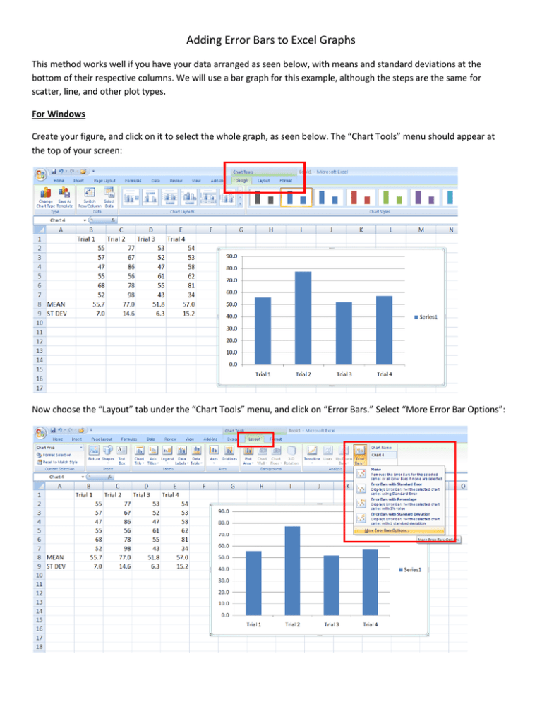
Adding Error Bars to Excel Graphs
This method works well if you have your data arranged as seen below, with means and standard deviations at the
bottom of their respective columns. We will use a bar graph for this example, although the steps are the same for
scatter, line, and other plot types.
For Windows
Create your figure, and click on it to select the whole graph, as seen below. The “Chart Tools” menu should appear at
the top of your screen:
Now choose the “Layout” tab under the “Chart Tools” menu, and click on “Error Bars.” Select “More Error Bar Options”:
The “Format Error Bars” box should now appear, as shown below. Choose whether you want your error bars to go up,
down, or both, by checking the appropriate buttons. To use your calculated standard deviation (or standard error)
values for your error bars, click on the “Custom” button under “Error Amount” and click on the “Specify Value” button.
The small “Custom Error Bars” dialog box will then appear, asking you to specify the value(s) of your error bars.
Now, move the cursor over your spreadsheet data and select the cells that contain your standard deviation calculations
(see below). By default, these values will be entered as “Positive Error Value”, and positive error bars will be created. If
you want error bars that go in both directions, you will also have to repeat this step for the “Negative Error Value”.
Click on “OK” and enjoy your beautiful new error bars:
For Mac
Create your figure, and click on it to select the whole graph, as seen below. The “Chart Layout” menu should appear.
Click on “Error Bars” and the “Error Bars Options” as shown below.
The “Format Error Bars” box should now appear, as shown below left. Choose whether you want your error bars to go
up, down, or both, by checking the appropriate buttons. To use your calculated standard deviation (or standard error)
values for your error bars, click on the “Custom” button under “Error Amount” and click on the “Specify Value” button.
The small “Custom Error Bars” dialog box will then appear, asking you to specify the value(s) of your error bars.
Select the “Positive Error Value” box, and move the cursor over your spreadsheet data and select the cells that contain
your standard deviation calculations (see above). If you want error bars that go in both directions, you will also have to
repeat this step for the “Negative Error Value”.
Click on “OK” and enjoy your beautiful new error bars: